Which Excel versions support dynamic array functions?

Dynamic array functions are supported in Excel for Microsoft 365 and Excel 2021 or later versions.

Can I use dynamic arrays with large datasets?

Yes, dynamic arrays are efficient and can handle large datasets faster than traditional array formulas.

How do I avoid #SPILL! errors when using dynamic arrays?

Ensure that the spill range is clear of data or formatting that could block the array from spilling into adjacent cells.

Can dynamic arrays replace older array formulas?

Yes, dynamic arrays simplify many tasks previously done with complex Ctrl+Shift+Enter array formulas.

Dynamic Arrays for Data Analysis June 9, 2026

Using Excel Dynamic Array Functions for Efficient Data Analysis

Q: What are dynamic arrays in Excel?

Dynamic arrays in Excel are formulas that return multiple values which spill into adjacent cells automatically, simplifying data manipulation.

Introduction

Excel has been an indispensable tool for data analysis for decades. With the introduction of dynamic array functions, it has become even more powerful and efficient. Dynamic arrays allow formulas to return multiple values that spill into adjacent cells automatically, simplifying complex data manipulation tasks. This article explores how you can leverage dynamic arrays for data analysis in Excel to save time, reduce errors, and improve your workflow.

What Are Dynamic Arrays in Excel?

Dynamic arrays are a new way Excel handles formulas that return multiple values. Traditionally, Excel formulas returned a single value per cell, and handling arrays required special array formulas entered with Ctrl+Shift+Enter. Dynamic arrays eliminate this complexity by automatically spilling results into adjacent cells. This functionality is available in Excel 365 and Excel 2021.

Some of the most popular dynamic array functions include:

FILTER – Extracts data that meet specified criteria.
SORT – Sorts data in ascending or descending order.
UNIQUE – Returns a list of unique values.
SEQUENCE – Generates a sequence of numbers.
RANDARRAY – Creates an array of random numbers.
XLOOKUP – A modern lookup function that supports dynamic arrays.

Benefits of Using Dynamic Arrays for Data Analysis in Excel

Dynamic arrays bring several benefits to data analysis:

Automatic Spill: No need to manually select ranges or use complex array formulas.
Improved Readability: Formulas are simpler and easier to understand.
Efficiency: Faster calculations for large datasets.
Flexibility: Easily handle changing data sizes without adjusting formulas.

Practical Examples of Dynamic Array Functions for Data Analysis

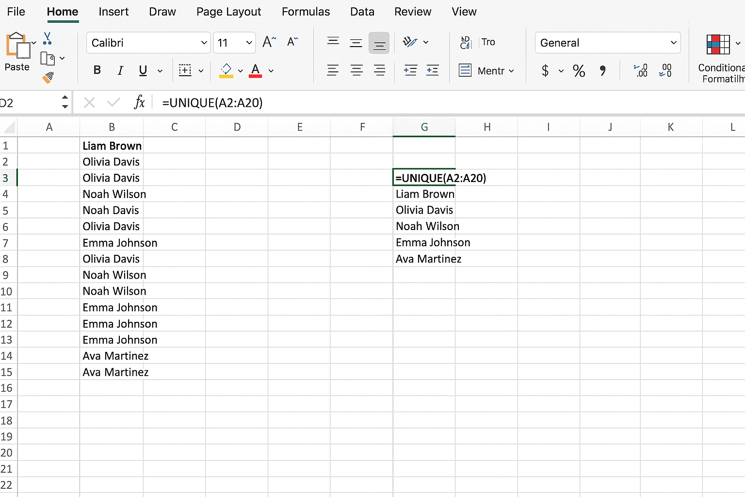
1. Extracting Unique Values with UNIQUE

Suppose you have a list of sales representatives’ names with duplicates and want to get a unique list.

=UNIQUE(A2:A20)

This formula returns a spilled array of unique names from the range A2:A20.

2. Filtering Data with FILTER

You want to extract all sales transactions greater than $1000 from a table with sales amounts in column C.

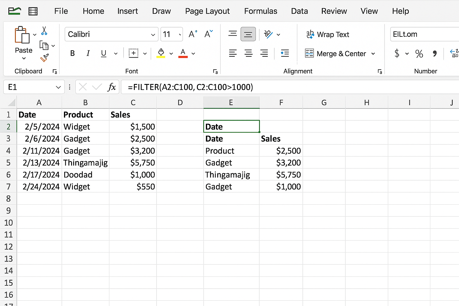
=FILTER(A2:C100, C2:C100>1000)

This returns all rows where the sales amount exceeds $1000.

3. Sorting Data with SORT

To sort a list of product names in column A alphabetically:

=SORT(A2:A50)

This spills the sorted list into cells below.

4. Combining UNIQUE and SORT

To get a sorted list of unique product categories:

=SORT(UNIQUE(B2:B100))

This returns a sorted array of unique categories from column B.

5. Generating Sequential Numbers with SEQUENCE

To create a list of numbers from 1 to 20:

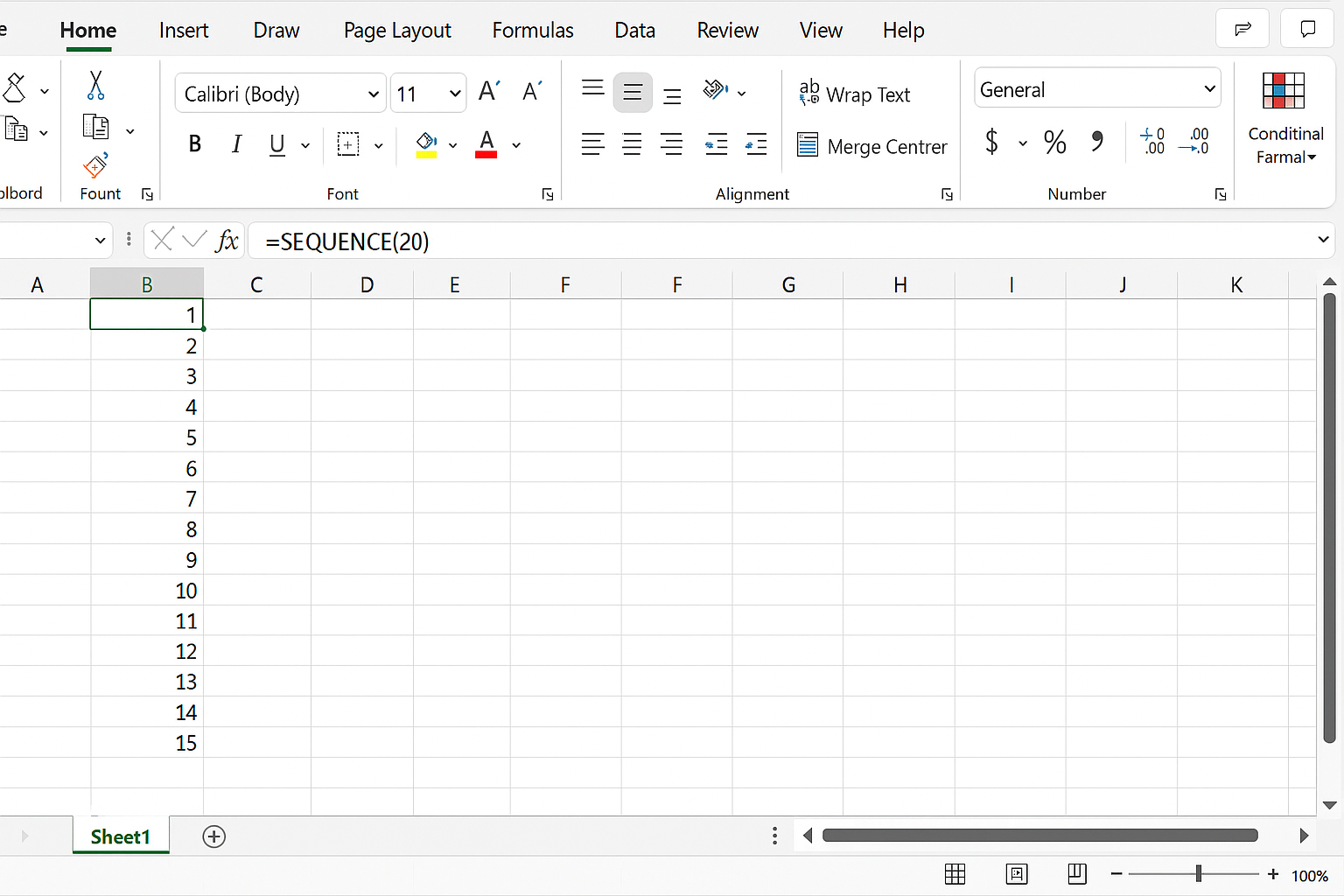
=SEQUENCE(20)

This spills numbers 1 through 20 into 20 rows.

6. Using XLOOKUP with Dynamic Arrays

To lookup multiple product prices based on a list of product IDs in column E:

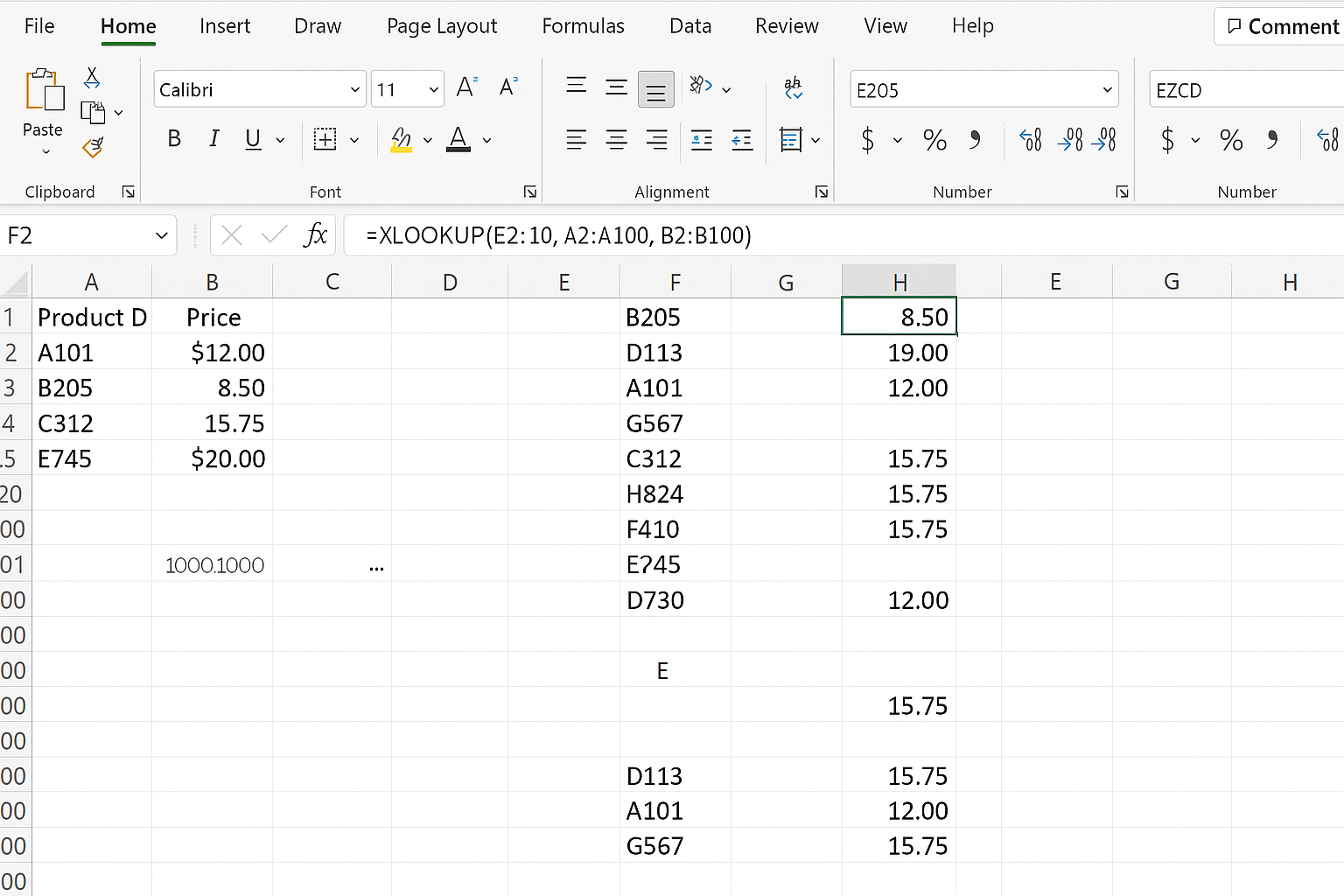
=XLOOKUP(E2:E10, A2:A100, B2:B100)

This returns prices for all product IDs in E2:E10.

Tips for Using Dynamic Arrays Effectively

Be mindful of spill ranges: Ensure there are blank cells where the array can spill; otherwise, you will get a #SPILL! error.
Combine functions: Nest functions like FILTER, SORT, and UNIQUE for powerful data manipulation.
Use named ranges: Improves formula readability and reduces errors.
Check compatibility: Dynamic arrays work only in newer Excel versions (365, 2021).

FAQ

Data Analysis Dynamic Arrays Excel Excel Functions Spreadsheet Tips