Mastering Excel Data Transformation: A Complete Guide to Unpivoting with Power Query
Introduction
Excel users frequently encounter datasets arranged in wide or horizontal formats that limit analysis options. Whether you receive monthly sales figures across columns or survey responses spread horizontally, transforming this data into a normalized, vertical layout is essential. This process, called unpivoting, converts columns of data points into rows, enabling more effective use of PivotTables, filtering, and formulas.
In this comprehensive guide, you will learn how to unpivot Excel data using Power Query, a powerful Excel tool designed for data transformation and automation. We will provide step-by-step instructions, practical examples, and tips to improve your spreadsheet productivity and data analysis capabilities.
What is Unpivoting and Why Use It?
Unpivoting flips your data from a horizontal format to a vertical one. For example, a table with months as column headers and sales as values can be unpivoted so that each sale is listed with the month in a single row. This normalized structure makes it easier to summarize data using PivotTables, apply formulas uniformly, or connect to other datasets.
Benefits of unpivoting include:
- Creating better source data for flexible PivotTables
- Simplifying calculations by consistent row-based data
- Facilitating data integration and analysis
- Automating repetitive data reshaping tasks
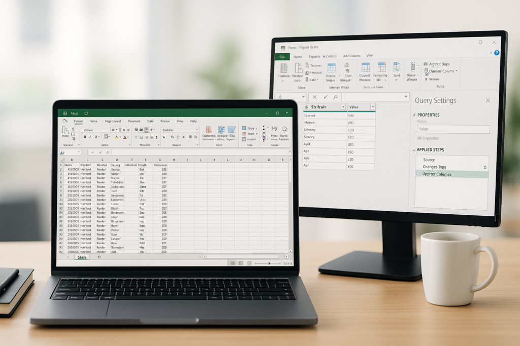
Getting Started with Power Query in Excel
Power Query is built into Excel 2016 and later versions and available as an add-in for Excel 2010 and 2013. It provides an intuitive interface for importing, cleaning, and transforming data without complex formulas.
To open Power Query:
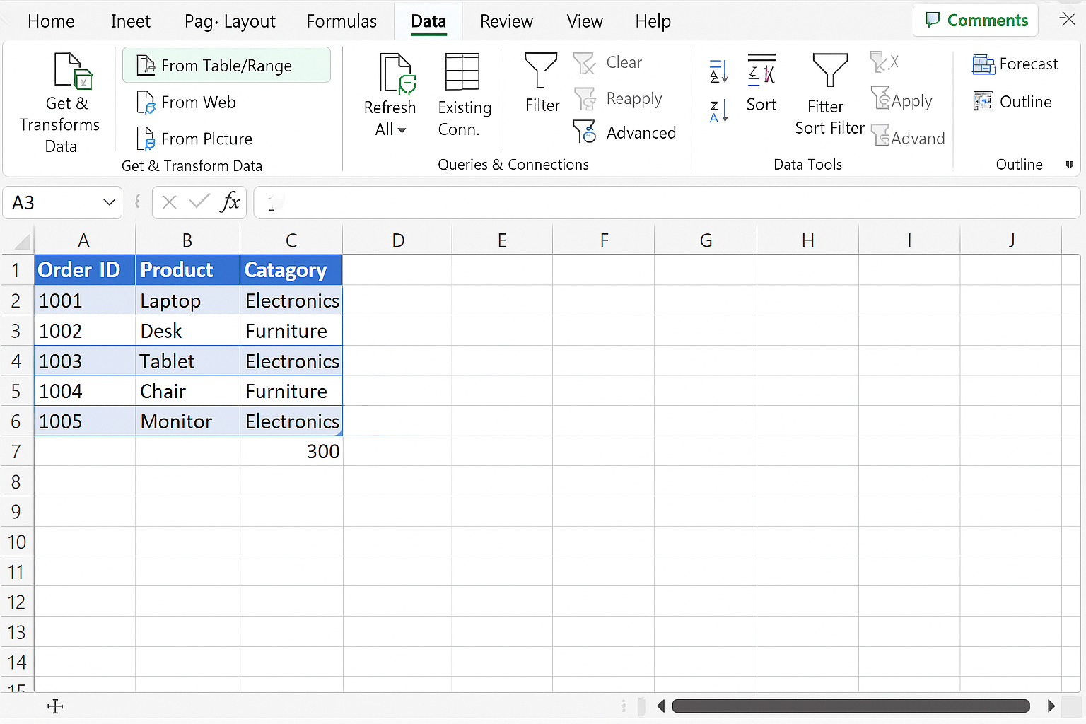
- Go to the Data tab on the Excel ribbon.
- Click Get & Transform Data group, then select From Table/Range (ensure your data is formatted as a table or select the range).
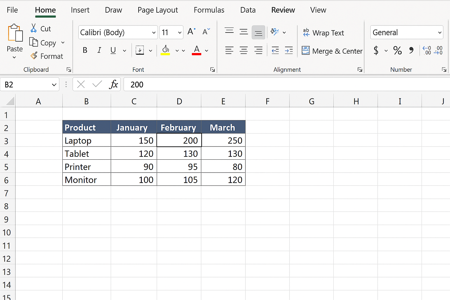
Hands-On Example: Unpivoting Monthly Sales Data
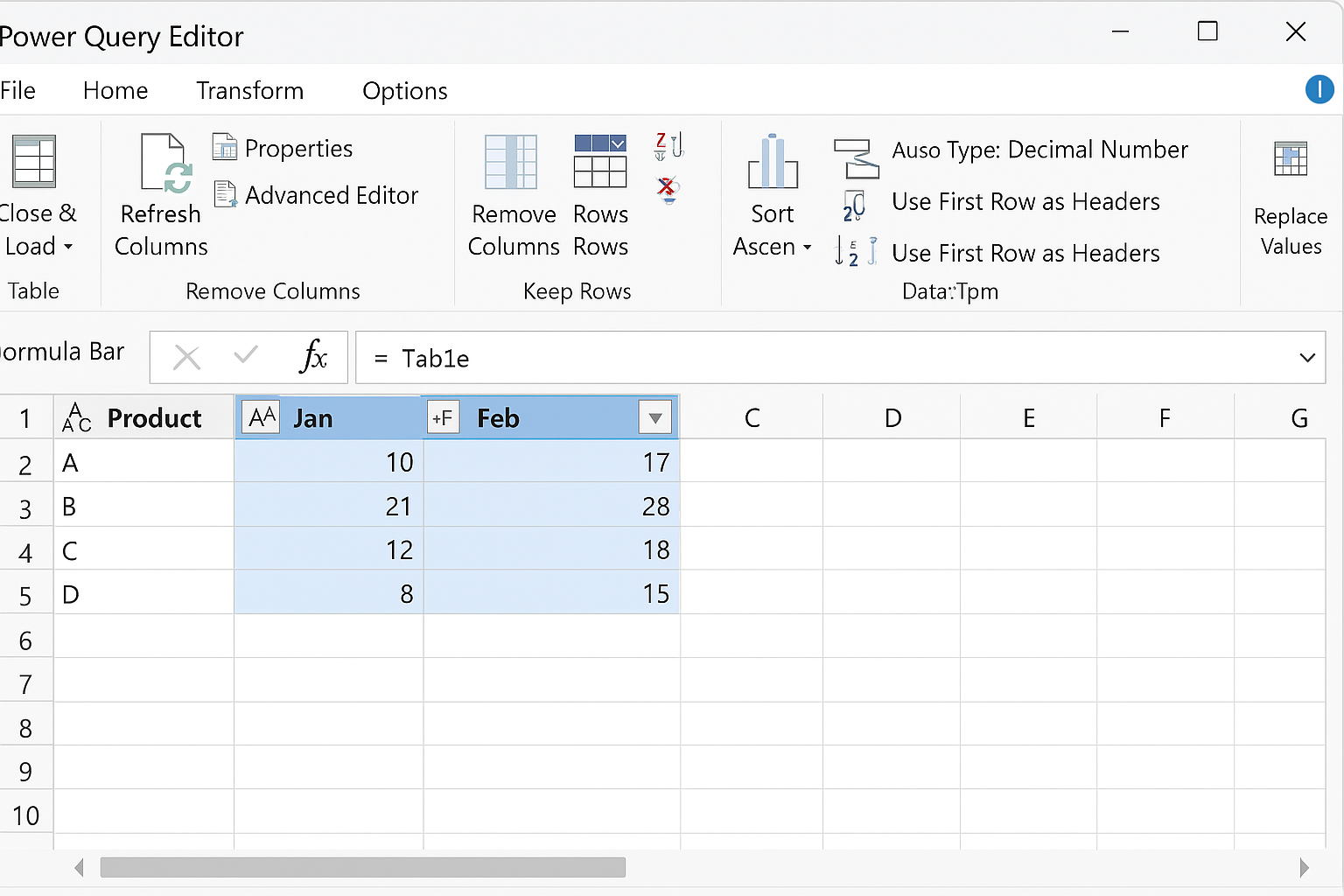
Consider a dataset showing sales per product across months in a horizontal layout:
| Product | Jan | Feb | Mar |
|---|---|---|---|
| Widget A | 120 | 135 | 150 |
| Widget B | 200 | 190 | 210 |
Our goal is to unpivot the months so that each row contains Product, Month, and Sales.
Step-by-Step Unpivoting
-
- Select your data range: Click anywhere inside your data table.
-
- Load into Power Query: On the Data tab, click From Table/Range. Excel opens the Power Query Editor.
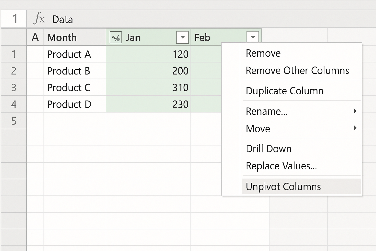
- Identify columns to unpivot: In the Power Query Editor, select the Jan, Feb, and Mar columns by clicking their headers while holding Ctrl.
- Apply Unpivot: Right-click on any selected month column header, then choose Unpivot Columns from the context menu.
-
- Rename columns: Power Query creates two columns named Attribute and Value. Double-click Attribute and rename it to Month. Rename Value to Sales.
- Change data types: Ensure Sales is set as a number by clicking the icon next to the column header and selecting Whole Number or Decimal Number.
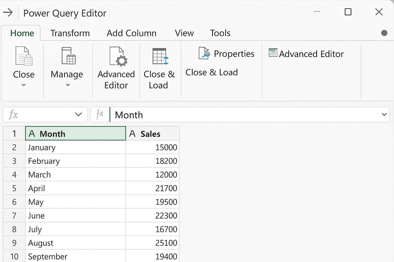
- Load transformed data back to Excel: Click Close & Load on the Home tab to create a new worksheet with the unpivoted data.
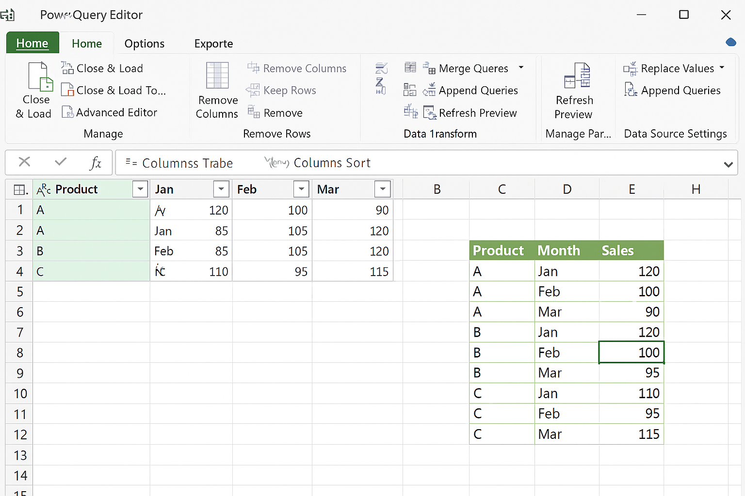
Resulting Table
| Product | Month | Sales |
|---|---|---|
| Widget A | Jan | 120 |
| Widget A | Feb | 135 |
| Widget A | Mar | 150 |
| Widget B | Jan | 200 |
| Widget B | Feb | 190 |
| Widget B | Mar | 210 |
Advanced Tips for Efficient Unpivoting
- Dynamic column selection: If your dataset has many columns, select the columns you want to keep (e.g., Product) and choose Unpivot Other Columns instead of Unpivot Columns. This way, any new months added later will auto-include.
- Handling blank or null values: Use the Power Query filter to remove rows with null or blank sales for cleaner reports.
- Automate refresh: After loading, refresh the query whenever your source data changes by right-clicking the query table and selecting Refresh.
- Combine with other transformations: Power Query supports merging, splitting columns, and calculated columns before or after unpivoting for comprehensive data prep.
Using Unpivoted Data for Powerful PivotTables
Once data is unpivoted, creating a PivotTable is straightforward and much more flexible:
- Select any cell in the unpivoted table.
- Go to the Insert tab and click PivotTable.
- Choose where to place the PivotTable (new worksheet or existing).
- Add fields like Product to Rows, Month to Columns, and Sales to Values.
This setup enables dynamic analysis such as monthly trends, product comparisons, and filtering by months or products with ease.
FAQ
What versions of Excel support Power Query?
Power Query is integrated in Excel 2016 and later. For Excel 2010 and 2013, you can install Power Query as a free add-in from Microsoft’s website.
Can I unpivot data with formulas instead of Power Query?
While formulas like INDEX, OFFSET, or VBA macros can imitate unpivoting, Power Query simplifies the task with a user-friendly interface and better performance, especially for large datasets.
How do I update my unpivoted data when the source changes?
Simply click inside the unpivoted table, right-click, and select Refresh. Power Query will rerun the transformation on updated source data.
Can I unpivot data from external sources like CSV or databases?
Yes. Power Query supports importing from CSV, databases, web pages, and many other sources. Once imported, you can apply the same unpivot steps.
What if my data has multiple header rows?
You’ll need to clean your data first by removing extra header rows or promoting headers correctly within Power Query before unpivoting.
Conclusion
Unpivoting data in Excel is a crucial skill for transforming cumbersome horizontal datasets into structured, analyzable tables. Power Query provides a robust and easy-to-use solution for this task, boosting your productivity and analytical capabilities. By following the step-by-step instructions and tips in this guide, you can confidently reshape your data, automate repetitive tasks, and create insightful reports with PivotTables.
Practice unpivoting different datasets to unlock the full power of Excel for data analysis and automation.
Want practical Excel help?
Support free Excel tutorials, get weekly tips, or contact us for Excel programming, VBA, Power Query, dashboards, and automation work.