How to Prepare Your Data for Creating Effective Pivot Tables

Introduction
Pivot tables are one of the most powerful features in Excel, allowing users to summarize, analyze, and visualize large datasets quickly. However, the key to creating effective pivot tables lies in how well you prepare your data beforehand. Proper data preparation ensures that your pivot table will work smoothly, provide accurate results, and be easy to manipulate. In this article, we will explore the essential steps to prepare data for a pivot table, complete with practical examples and tips to make your Excel work more efficient.
What is a Pivot Table?
A pivot table is a data summarization tool that allows you to reorganize and extract meaningful information from a large dataset. It works by aggregating data, such as sums, averages, counts, or percentages, based on categories or fields you define. This makes pivot tables incredibly useful for business reports, data analysis, and decision-making.
Why Is Data Preparation Important?
Data preparation is crucial because pivot tables rely on clean, organized data. If data is incomplete, inconsistent, or poorly structured, the pivot table will produce incorrect or misleading summaries. Preparing your data ensures that you avoid errors, improve accuracy, and save time when building your pivot table.
Steps to Prepare Data for Pivot Table
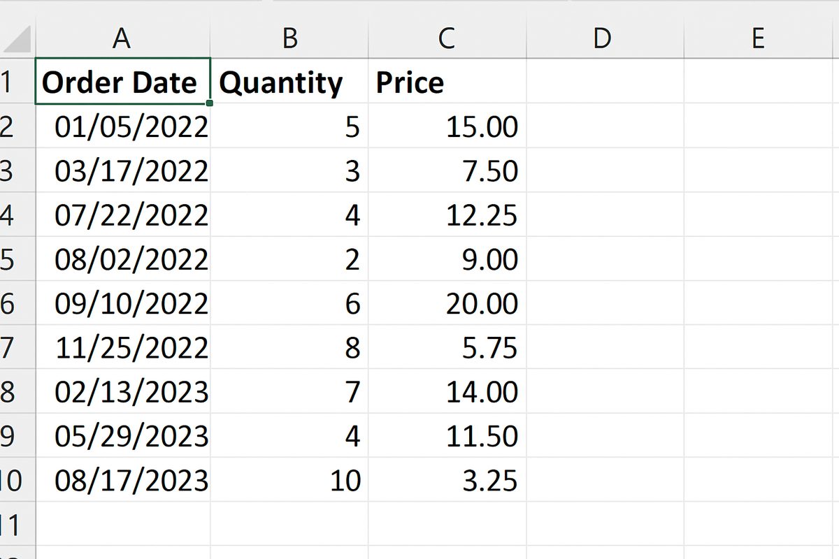
1. Organize Data in a Tabular Format
The first step is to ensure your data is arranged in a table format with rows and columns. Each column should have a clear, unique header describing the data it contains. Avoid merging cells or creating blank rows and columns within the dataset.
Example:
| Order ID | Product | Category | Quantity | Price | Order Date |
|---|---|---|---|---|---|
| 1001 | Desk Chair | Furniture | 2 | 85 | 2024-03-01 |
| 1002 | Notebook | Stationery | 5 | 2.5 | 2024-03-02 |
2. Remove Blank Rows and Columns
Ensure there are no blank rows or columns inside your dataset. Blank rows or columns can cause the pivot table to interpret your data incorrectly or limit the range of data it includes.
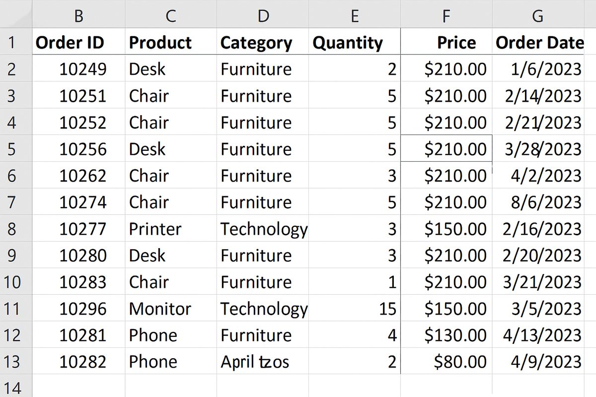
3. Use Consistent Data Types in Columns
Each column should contain the same type of data. For example, a “Quantity” column should only have numbers, and a “Date” column should contain dates. Mixing data types can lead to errors or prevent Excel from summarizing the data correctly.
4. Avoid Subtotals and Totals Inside Data
Your raw data should not include any subtotal or total rows or columns. Pivot tables calculate these automatically based on your selections, so including them in the source data can cause duplication or inaccurate summaries.
5. Format Dates Properly
If your dataset includes dates, make sure they are in a proper date format recognized by Excel. This allows you to group data by months, quarters, or years easily when creating the pivot table.
6. Use Meaningful and Unique Headers
Headers should be descriptive but concise. Avoid special characters that might cause issues, and ensure each column has a unique header. For example, use “Order Date” instead of just “Date” if there are multiple date fields.
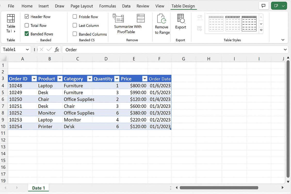
7. Convert Data Range to an Excel Table
Converting your data range to an Excel Table (using Insert > Table) offers several benefits:
- Dynamic data range: The table automatically expands as you add new data.
- Improved readability and filtering options.
- Easy reference for pivot table source data.
8. Check for Duplicates and Errors
Scan your dataset for duplicate rows or errors that might skew your pivot table results. Use Excel’s built-in tools such as Remove Duplicates or Data Validation to maintain data integrity.
Practical Example: Preparing Sales Data for Pivot Table
Imagine you have the following sales data in Excel:
| Order ID | Product | Category | Quantity | Price | Order Date |
|---|---|---|---|---|---|
| 1001 | Desk Chair | Furniture | 2 | 85 | 2024-03-01 |
| 1002 | Notebook | Stationery | 5 | 2.5 | 2024-03-02 |
| 1003 | Pen | Stationery | 10 | 1.2 | 2024-03-02 |
Steps to prepare this data:
- Remove the blank row at the bottom.
- Ensure each column’s data type is consistent (e.g., numbers in Quantity and Price, dates in Order Date).
- Convert the range to an Excel Table for easy management.
- Check for duplicates or erroneous entries.
- Make sure headers are clear and unique.
Creating the Pivot Table
Once the data is prepared, select any cell inside the table, then go to Insert > PivotTable. Excel will automatically select the entire table as the data source. From there, you can drag and drop fields into the Rows, Columns, Values, and Filters areas to build your pivot table.
Common Mistakes to Avoid When Preparing Data
- Including blank rows or columns: These interrupt the data range and may cause incomplete pivot tables.
- Mixing data types in a single column: This confuses Excel’s aggregation functions.
- Using merged cells: Pivot tables do not handle merged cells properly.
- Inconsistent date formats: This prevents grouping by date periods.
- Including subtotals or totals in raw data: Causes double counting.
Conclusion
Preparing your data correctly is the foundation of creating effective pivot tables in Excel. By organizing your data in a clean tabular format, using consistent data types, removing blanks and duplicates, and converting your data into an Excel Table, you ensure accurate, flexible, and insightful pivot table reports. Taking the time to prepare your data properly saves you time and frustration later and maximizes the power of your Excel pivot tables.
Related Articles
- Pivot Tables Tutorial: A Beginner’s Guide to Summarizing Data
- What Is a Pivot Table and How Can It Help You Analyze Data?
- How to Create a Pivot Table in Excel Step-by-Step
- Understanding Pivot Table Fields: Rows, Columns, Filters, and Values Explained
- Advanced Pivot Table Techniques to Master Data Analysis
Want practical Excel help?
Support free Excel tutorials, get weekly tips, or contact us for Excel programming, VBA, Power Query, dashboards, and automation work.