How to Use the Excel FILTER Function with Dynamic Arrays
Introduction
The Excel FILTER function is one of the most powerful tools introduced with Excel’s dynamic array functions. It allows users to extract data that meets specific criteria dynamically, making spreadsheets more interactive and easier to analyze. This article will explore how to use the Excel FILTER function effectively with practical examples and tips.
What is the Excel FILTER Function?
The Excel FILTER function returns an array that meets the criteria you specify. Unlike traditional filtering, this function outputs dynamic arrays that spill into adjacent cells automatically, updating as source data changes.
Syntax:
FILTER(array, include, [if_empty])
- array: The range or array to filter.
- include: A Boolean array, where TRUE values indicate which rows or columns to include.
- if_empty: Optional. The value to return if no entries meet the criteria.
Advantages of Using the FILTER Function
- Dynamic output: Automatically spills filtered results into multiple cells.
- Easy to update: Automatically refreshes as source data or criteria change.
- Flexible criteria: Can use complex logical conditions.
- Improves readability: Keeps formulas simple compared to older array formulas.
Practical Examples of the Excel FILTER Function
Example 1: Filtering a List by One Criterion
Suppose you have a list of employees with departments and salaries:
| Name | Department | Salary |
|---|---|---|
| John | Sales | 50000 |
| Mary | Marketing | 60000 |
| Steve | Sales | 55000 |
| Linda | IT | 70000 |
To filter only employees from the Sales department, use:
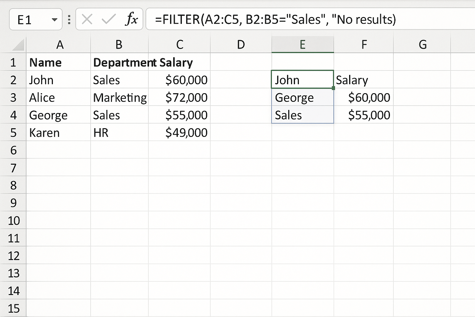
=FILTER(A2:C5, B2:B5="Sales", "No results")
This formula will return all rows where the Department is “Sales”. If no match is found, it returns “No results”.
Example 2: Filtering with Multiple Criteria
To get employees from Sales department with salary over 52000:
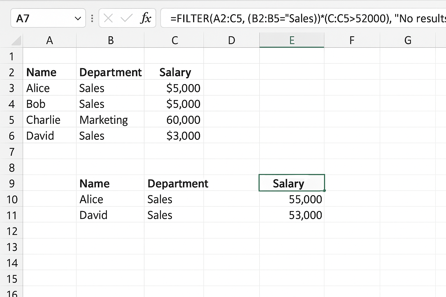
=FILTER(A2:C5, (B2:B5="Sales")*(C2:C5>52000), "No results")
Here, the multiplication operator acts as an AND condition combining the two criteria.
Example 3: Filtering Unique Values
You can combine FILTER with UNIQUE to get distinct filtered results. For example, to get unique departments with salaries greater than 55000:
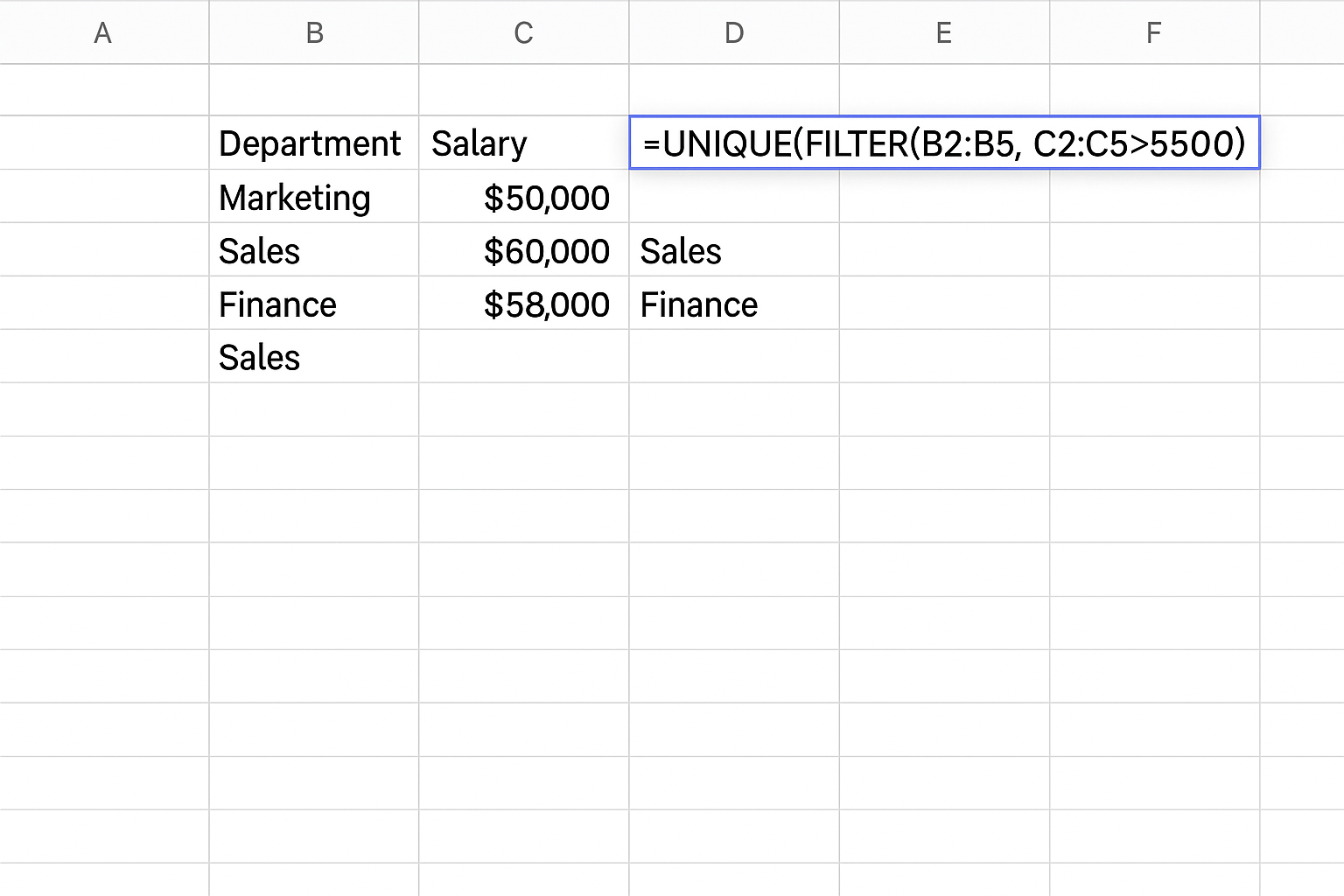
=UNIQUE(FILTER(B2:B5, C2:C5>55000))
Example 4: Using FILTER with Dates
Suppose you have sales data including dates and amounts:
| Date | Sales |
|---|---|
| 2024-01-01 | 1200 |
| 2024-02-01 | 1500 |
| 2024-01-15 | 1100 |
| 2024-03-01 | 1700 |
To filter sales from January 2024:
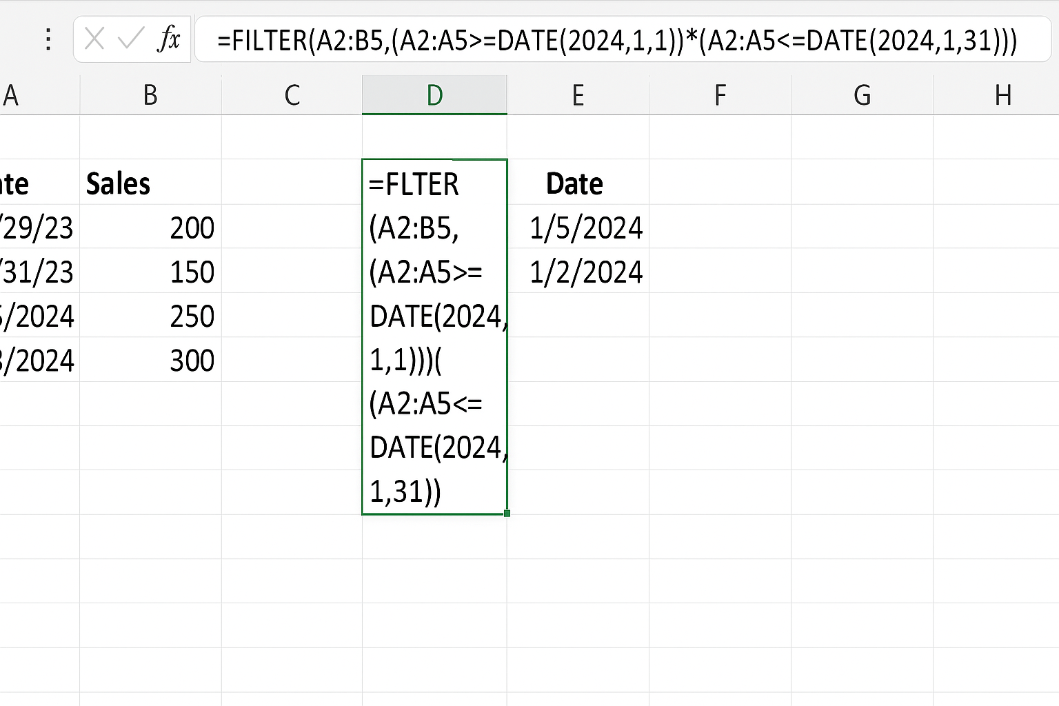
=FILTER(A2:B5, (A2:A5>=DATE(2024,1,1))*(A2:A5<=DATE(2024,1,31)))
Tips for Using FILTER with Dynamic Arrays
- Ensure enough empty cells below the formula for the spill range.
- Use named ranges or Excel tables for easier references.
- Combine FILTER with other dynamic array functions like SORT, UNIQUE, and SEQUENCE for more powerful results.
- Use logical operators like *, + for AND and OR conditions respectively.
Common Errors and How to Fix Them
- #CALC! error: Occurs if the spill area is blocked by other data. Clear cells below the formula.
- No results: Use the optional if_empty argument to display a message instead of an error.
- Incorrect criteria: Make sure your logical expressions return arrays of TRUE/FALSE.
FAQ
See the FAQ section below for common questions about the Excel FILTER function.
Conclusion
The Excel FILTER function is a versatile tool that leverages dynamic arrays to make filtering data easier, faster, and more flexible. Whether you are filtering by one criterion or multiple complex conditions, FILTER simplifies the process and enhances your spreadsheet capabilities. By mastering this function, you can create interactive reports and dashboards that update automatically as data changes.
Related Articles
- Understanding Dynamic Array Functions in Excel: A Beginner’s Guide
- Top Excel Dynamic Array Formulas You Should Know
- Mastering the Excel SORT Function Using Dynamic Arrays
- Using the UNIQUE Function in Excel to Extract Distinct Values with Dynamic Arrays
- Advanced Techniques: Nesting Dynamic Array Functions in Excel
Want practical Excel help?
Support free Excel tutorials, get weekly tips, or contact us for Excel programming, VBA, Power Query, dashboards, and automation work.