What is a pivot table in Excel?

A pivot table is a tool in Excel that summarizes, analyzes, and organizes data from a larger dataset, allowing users to extract meaningful insights quickly.

How do I create a pivot table in Excel?

You select the data range, go to the Insert tab, click PivotTable, choose where to place it, and then drag fields into Rows, Columns, Values, and Filters areas to build the table.

Can I update a pivot table after changing the source data?

Yes, you can refresh the pivot table by right-clicking it and selecting Refresh, which updates the table based on the latest source data.

What types of calculations can pivot tables perform?

Pivot tables can perform various calculations including sums, counts, averages, minimums, maximums, and percentages.

Are pivot tables suitable for large datasets?

Yes, pivot tables are designed to efficiently summarize and analyze large datasets, making them ideal for data-heavy tasks.

Pivot Tables Basics June 14, 2026

How to Create a Pivot Table in Excel Step-by-Step

Introduction

Pivot tables are one of the most powerful features in Microsoft Excel, enabling users to summarize, analyze, explore, and present large amounts of data quickly and effectively. Whether you are a beginner or an experienced Excel user, knowing how to create a pivot table can transform the way you handle data and generate meaningful insights.

In this comprehensive guide, we will walk you through the process of creating a pivot table step-by-step. We will cover everything from preparing your data to customizing your pivot table for better analysis. Plus, we’ll include practical examples to help you understand how pivot tables work in real-world scenarios.

What is a Pivot Table?

A pivot table is a data summarization tool in Excel that automatically sorts, counts, averages, or totals data stored in one table or spreadsheet and displays the results in a new table. It allows users to reorganize and group data dynamically, making it easier to analyze and compare different parts of the dataset.

Step 1: Prepare Your Data

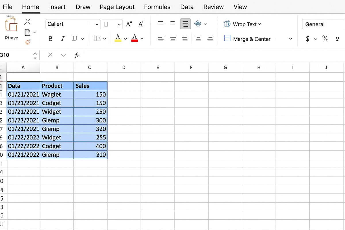
Before creating a pivot table, ensure your data is organized correctly:

Tabular format: Data should be in rows and columns with headers.
No blank rows or columns: Avoid empty rows or columns within your dataset.
Unique headers: Each column must have a clear and unique header.
Consistent data types: Data in each column should be of the same type (e.g., numbers, text, dates).

Example dataset:

Order ID	Product	Category	Sales	Region
1001	Smartphone	Electronics	699	North
1002	Laptop	Electronics	1200	South
1003	Tablet	Electronics	450	East
1004	Desk Chair	Furniture	150	North
1005	Bookshelf	Furniture	200	West

Step 2: Select Your Data Range

Click anywhere inside your data table. Excel will automatically detect the data range when creating the pivot table, but you can adjust it if needed.

Step 3: Insert the Pivot Table

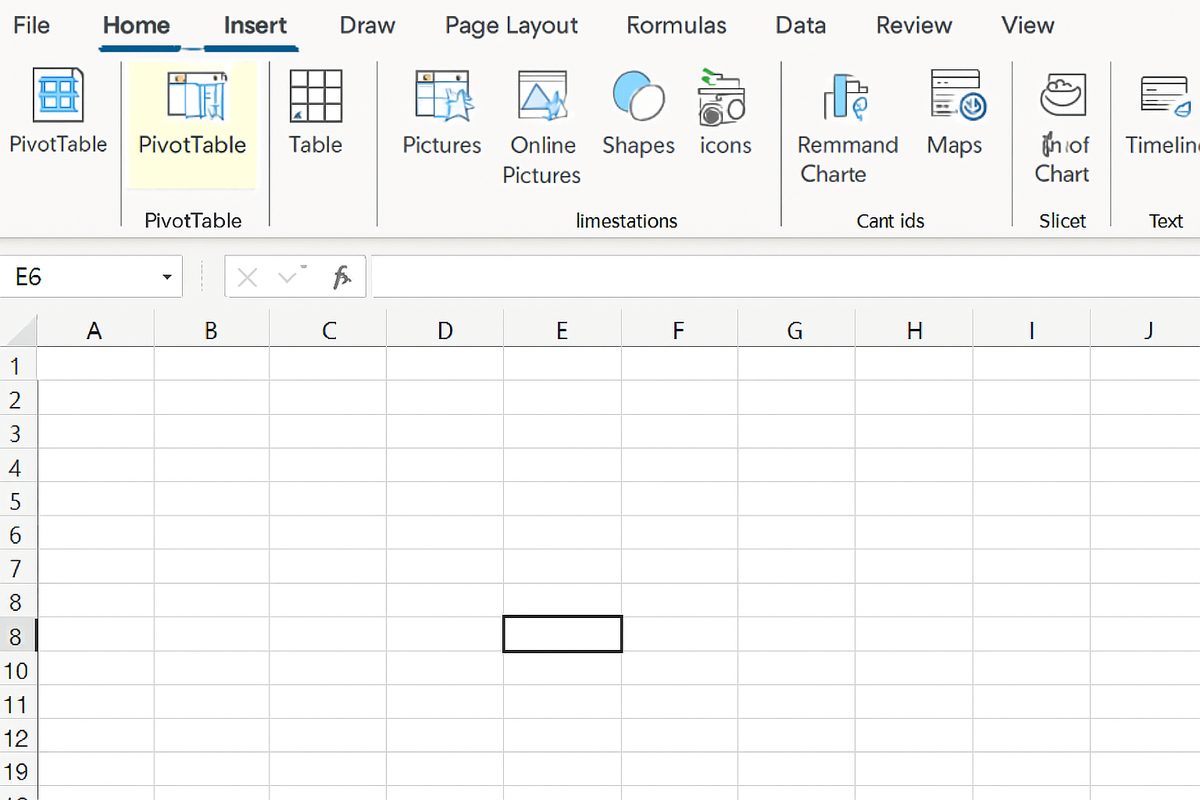
Follow these steps to insert a pivot table:

Go to the Insert tab on the Excel Ribbon.
Click on PivotTable.
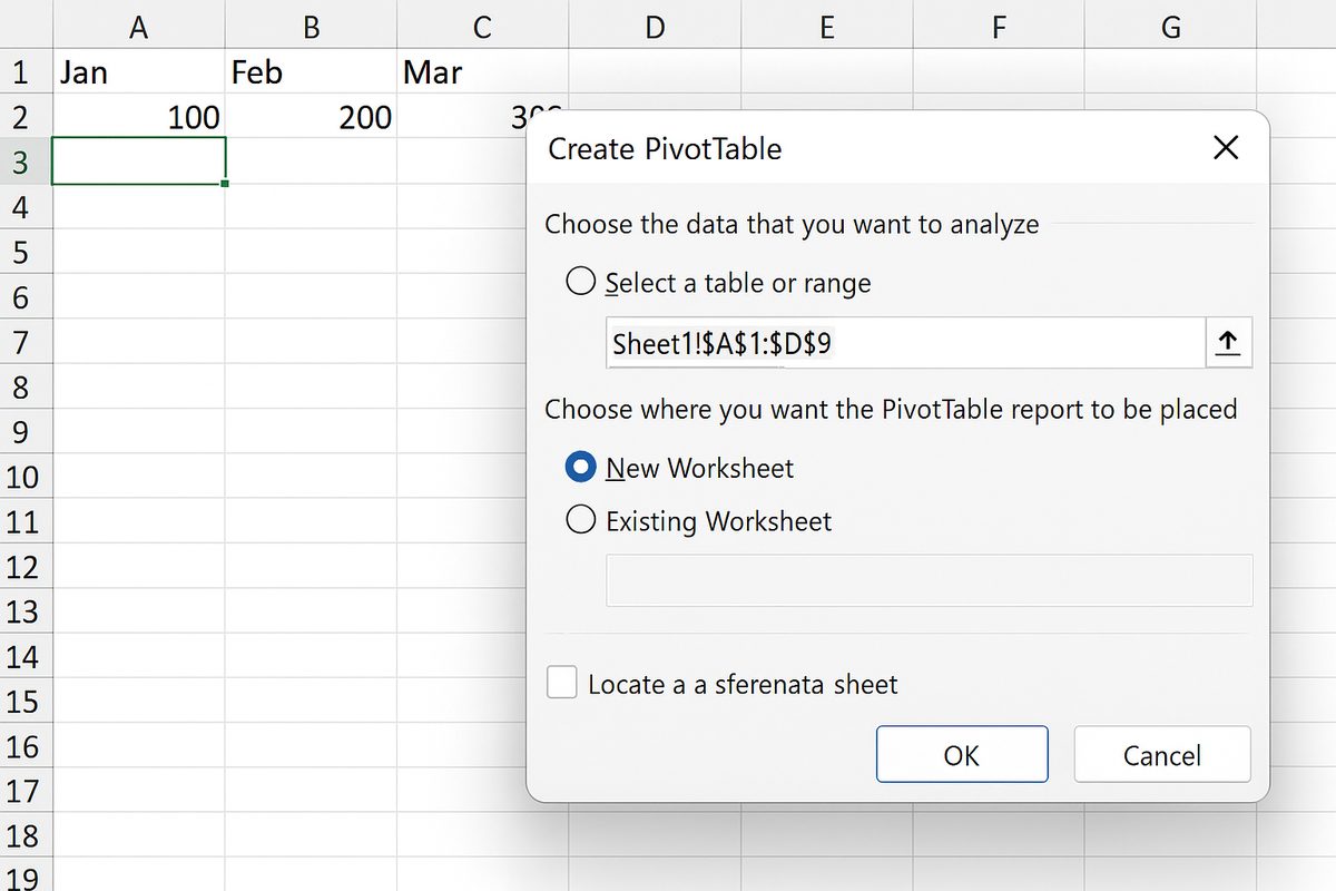
In the dialog box, confirm your data range.
Choose whether to place the pivot table in a new worksheet or an existing one.
Click OK.

Step 4: Build Your Pivot Table

Once the pivot table is inserted, you will see a blank pivot table frame and a PivotTable Fields pane with available columns from your data.

Drag and drop the fields into four areas:

Filters: Fields placed here allow you to filter the entire pivot table by specific criteria.
Columns: Fields here display as column headers in the pivot table.
Rows: Fields here display as row labels.
Values: These fields show the summarized data, such as sums, counts, or averages.

Example: To analyze total sales by category and region:

Drag Category to Rows.
Drag Region to Columns.
Drag Sales to Values (Excel will default to Sum of Sales).

Step 5: Customize Your Pivot Table

Excel offers multiple ways to customize your pivot table:

Change summary calculation: Click the dropdown next to the Values field > Value Field Settings > choose Sum, Count, Average, etc.
Sort and filter data: Use dropdown arrows on Row or Column labels to sort or filter data.
Group data: Right-click on date or numeric fields > Group to create custom groups.
Format numbers: Apply number formatting through Value Field Settings or Excel’s number format options.
Refresh data: If source data changes, right-click the pivot table > Refresh to update.

Practical Example: Sales Analysis Using Pivot Table

Imagine you want to analyze sales performance by product category and region from the example dataset above. Follow these steps:

Insert pivot table as described.
Place Category in Rows.
Place Region in Columns.
Place Sales in Values.

Your pivot table will display total sales for each category across different regions, helping you quickly identify top-performing areas or categories.

Tips for Working with Pivot Tables

Always keep your source data updated and clean.
Use meaningful field names for clarity.
Explore PivotTable Tools > Design and Analyze tabs for advanced options.
Leverage slicers and timelines for interactive filtering.
Practice with different datasets to gain confidence.

Conclusion

Creating pivot tables in Excel is an essential skill for anyone dealing with data analysis. By following the step-by-step instructions above, you can transform raw data into insightful summaries quickly and efficiently. Pivot tables help you save time, identify trends, and make data-driven decisions with ease.

Start practicing today by creating pivot tables with your own datasets, and explore the many customization options Excel offers to enhance your reports and dashboards.

Data Analysis Excel Excel tutorial Pivot Tables