How to Count Unique Items in Excel Pivot Tables Without Using the Data Model

Introduction
Counting unique items in Excel pivot tables is a common task for data analysis and reporting. However, if you are using Excel 2010 or earlier versions, or prefer not to use the Excel Data Model, you might find it challenging to count distinct values directly in pivot tables. This article explains how to count unique items in Excel pivot tables without relying on the Data Model, using simple formulas and practical techniques to enhance your spreadsheet productivity.
Why Count Unique Items?
Counting unique items, also known as distinct counts, helps you understand the diversity or variety of data entries within your dataset. For example, if you have a list of sales transactions with customer names, knowing how many unique customers made purchases is more insightful than just counting all transactions.
Limitations Without Data Model
Excel versions prior to 2013 or without Power Pivot support do not offer a built-in distinct count feature in pivot tables. This requires creative use of formulas and helper columns to achieve the same results.
Step-by-Step Guide: Count Unique Items Without Data Model
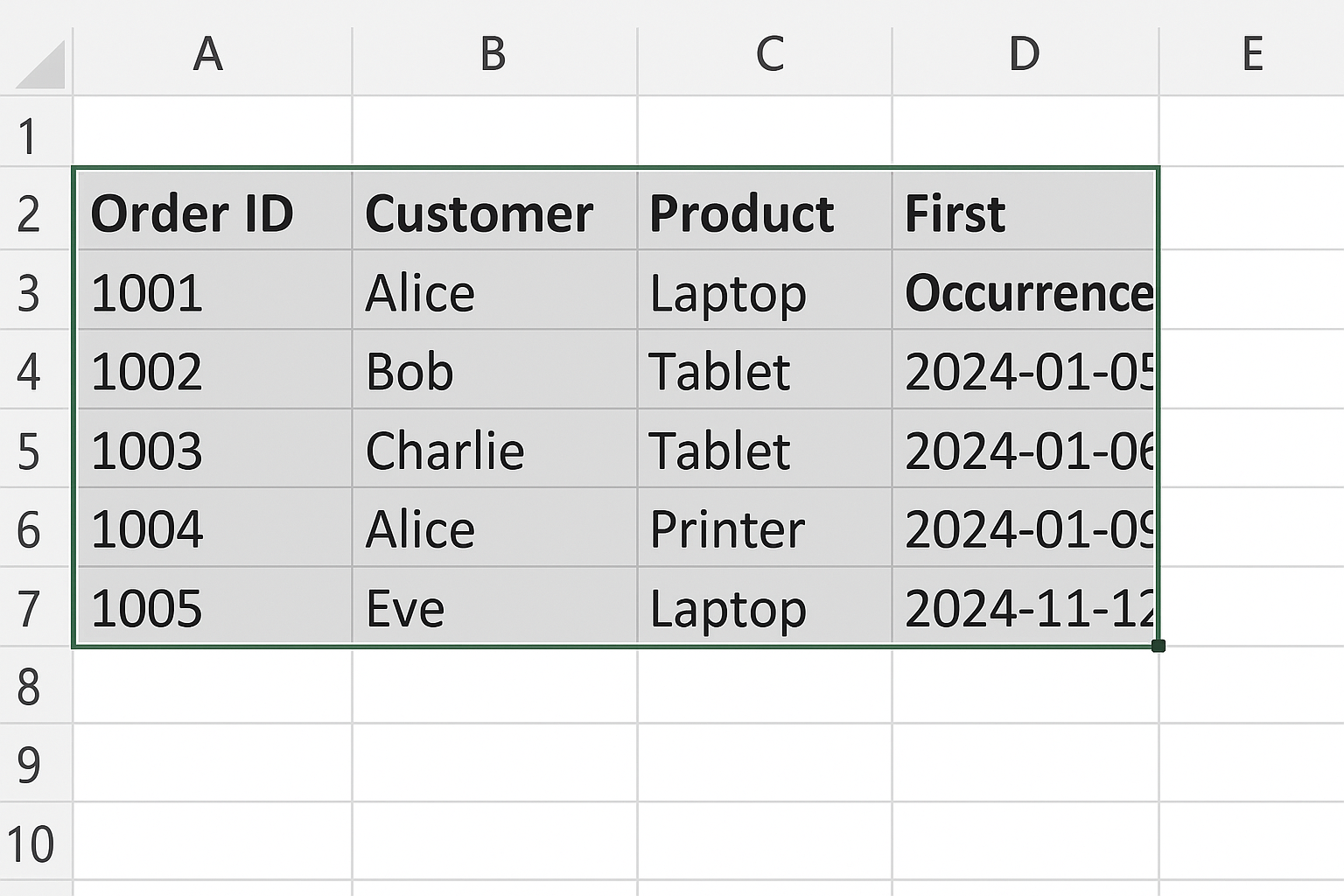
Step 1: Prepare Your Data
Assume you have a worksheet named SalesData with columns Order ID, Customer, and Product.
Example data:
| Order ID | Customer | Product |
|---|---|---|
| 1001 | John | Apples |
| 1002 | Mary | Bananas |
| 1003 | John | Oranges |
| 1004 | Steve | Apples |
| 1005 | Mary | Bananas |
Step 2: Add a Helper Column to Identify First Occurrences
Insert a new column titled First Occurrence next to your data.
In cell D2 (assuming your data starts at row 2), enter the formula to check if the customer is appearing for the first time:
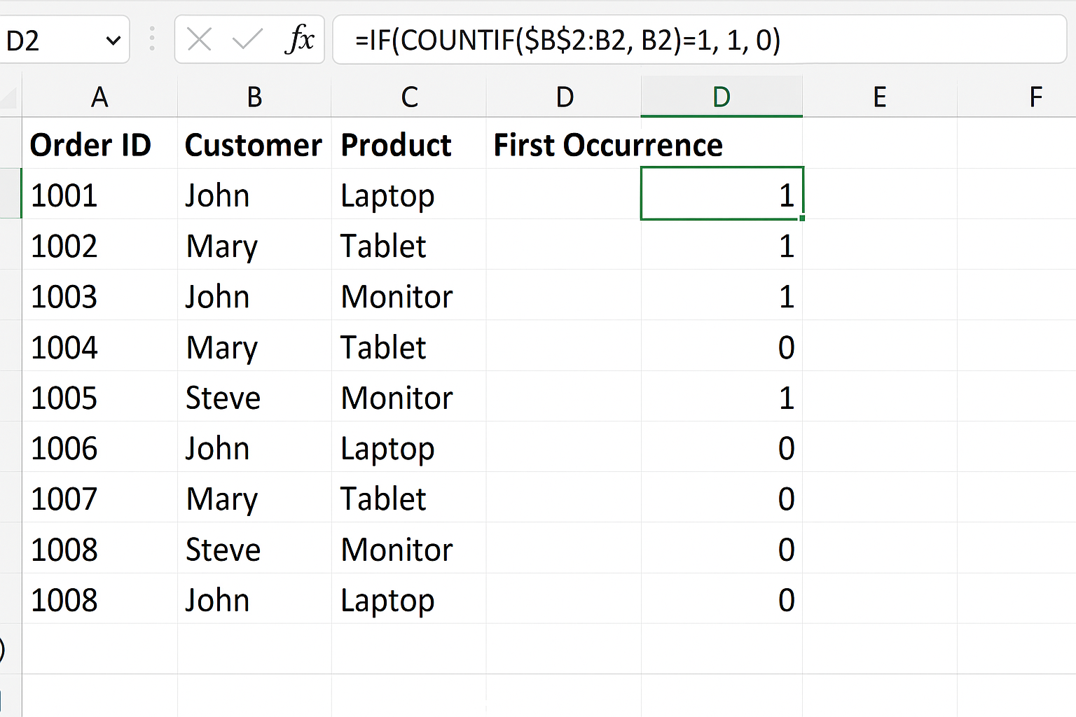
=IF(COUNTIF($B$2:B2, B2)=1, 1, 0)
This formula counts how many times the customer in current row has appeared from the top down to current row. If it is the first occurrence, it returns 1, otherwise 0.
Drag this formula down to cover all rows in your dataset.
Step 3: Create a Pivot Table
Select your entire data range including the new helper column (e.g., A1:D6).
Go to the Insert tab and click PivotTable.
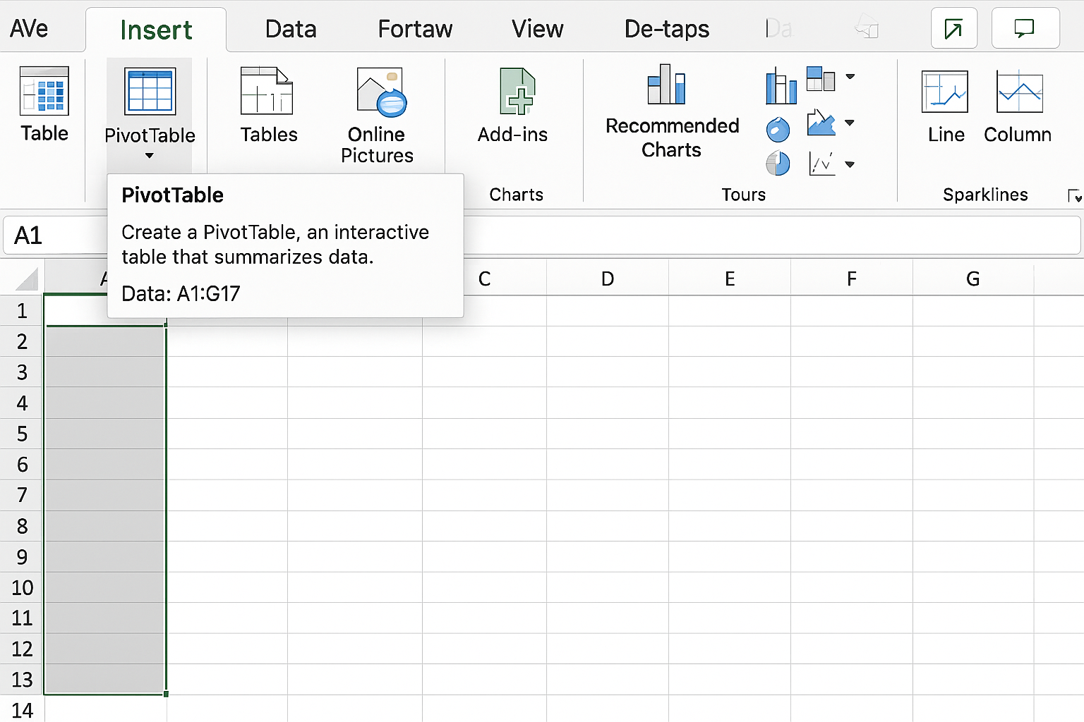
Choose to place the pivot table in a new worksheet or existing worksheet.
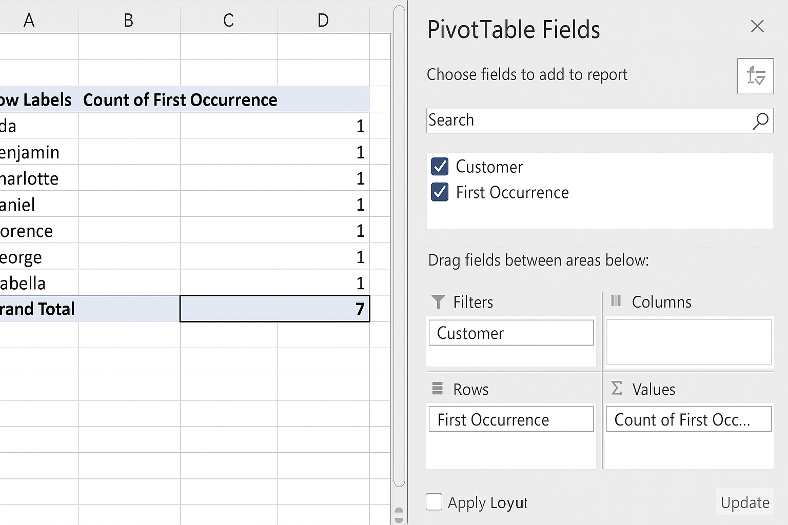
Step 4: Set Up the Pivot Table Fields
In the PivotTable Fields pane:
- Drag Customer to the Rows area.
- Drag First Occurrence to the Values area.
By default, the First Occurrence field will be summed, which counts the number of unique customers.
Step 5: Interpret the Results
The pivot table will display each customer as a row and a value of 1 next to their name. This indicates that each customer counts as one unique entry.
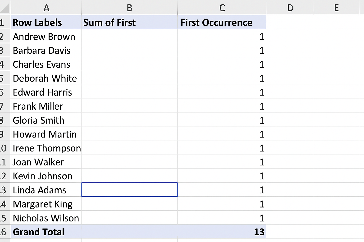
To get the total number of unique customers, check the grand total at the bottom of the pivot table’s values column.
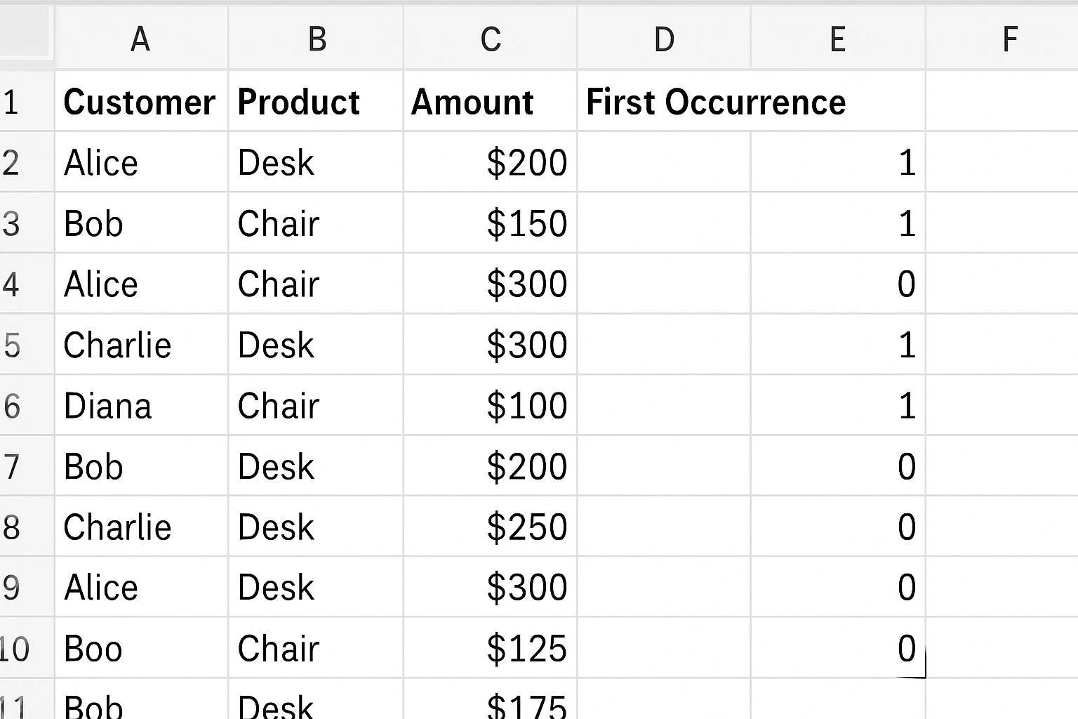
Example: Counting Unique Products per Customer
If you want to count how many unique products each customer purchased, you can modify the helper column formula as follows:
=IF(COUNTIFS($B$2:B2, B2, $C$2:C2, C2)=1, 1, 0)
This formula checks if the combination of customer and product appears for the first time up to the current row.
Update your pivot table by dragging Customer to Rows and First Occurrence to Values to see the count of unique products per customer.
Additional Tips for Productivity
- Named Ranges: Use named ranges for your data to make formulas more readable and pivot table ranges easier to update.
- Dynamic Ranges: Convert your data to an Excel Table (Ctrl + T) so that formulas and pivot tables update automatically as you add data.
- Formatting: Format your pivot table values as numbers with no decimal places for clarity.
- Sorting: Sort pivot table rows alphabetically or by count to better analyze your data.
Automation: Using VBA to Count Unique Items
If you frequently need to count unique items in pivot tables, consider automating the helper column insertion and pivot table refresh using VBA macros.
This can streamline repetitive tasks and reduce manual errors.
FAQ
Can I count unique items in pivot tables without helper columns?
In Excel versions 2013 and later, you can use the Data Model feature to count unique items directly. Without it, helper columns are necessary.
Does this method work for large datasets?
Yes, but performance might slow down with very large datasets. Using Excel Tables and efficient formulas can help.
Can I count unique dates or numbers with this approach?
Yes, the same helper column technique applies to any data type where you want to count distinct values.
How do I count unique items across multiple columns?
You can concatenate multiple columns in a helper column and then apply the COUNTIF or COUNTIFS logic to count unique combinations.
Is there a formula alternative without pivot tables?
Yes, formulas like SUMPRODUCT, COUNTIF, or UNIQUE (in Excel 365) can be used to count unique values without pivot tables.
Conclusion
Counting unique items in Excel pivot tables without the Data Model can be achieved efficiently using helper columns and simple formulas. This technique is compatible with older Excel versions and provides flexible ways to analyze distinct data points such as customers, products, or orders. By integrating these methods into your workflow, you can improve your data analysis capabilities and enhance productivity in Excel.