Mastering Excel Pivot Table Calculated Fields for Advanced Data Analysis

Pivot Tables are a powerful feature in Excel that allow you to summarize and analyze large datasets quickly. Calculated Fields enhance this functionality by enabling you to create new data fields based on existing ones, without altering your original dataset.

Understanding Calculated Fields

Calculated Fields let you perform custom calculations on your Pivot Table data. For example, you can calculate profit by subtracting costs from revenue directly within the Pivot Table.

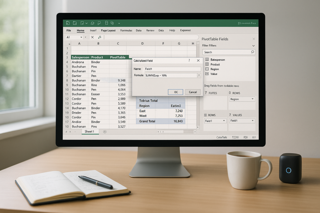
How to Insert a Calculated Field

To insert a Calculated Field, go to the PivotTable Analyze tab, click on Fields, Items & Sets, and select Calculated Field. Then, enter the formula using the existing field names.

Practical Step-by-Step: Creating a Calculated Field to Analyze Profit Margin

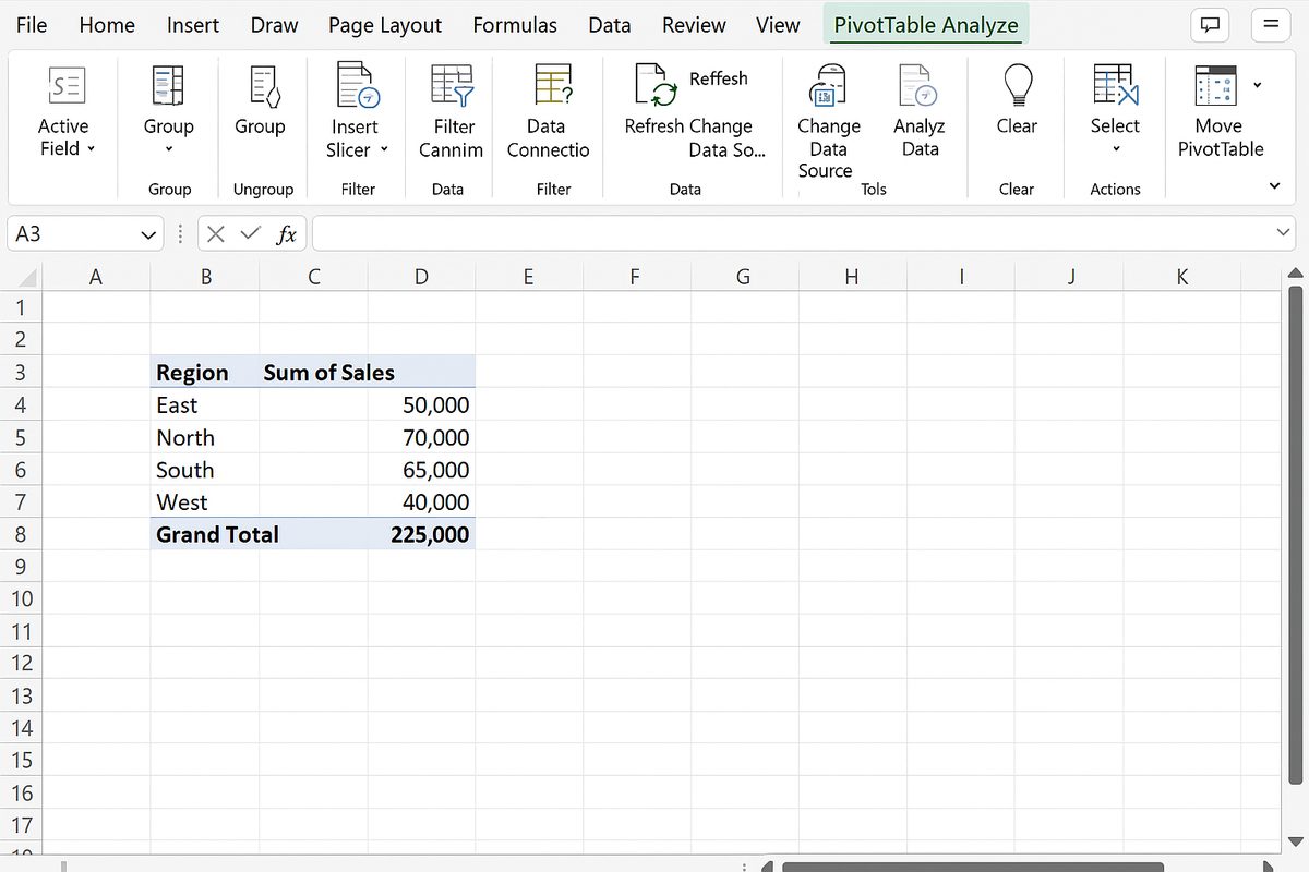
1. Click anywhere inside your Pivot Table to activate the PivotTable Tools on the ribbon.
2. Go to the PivotTable Analyze tab on the ribbon.



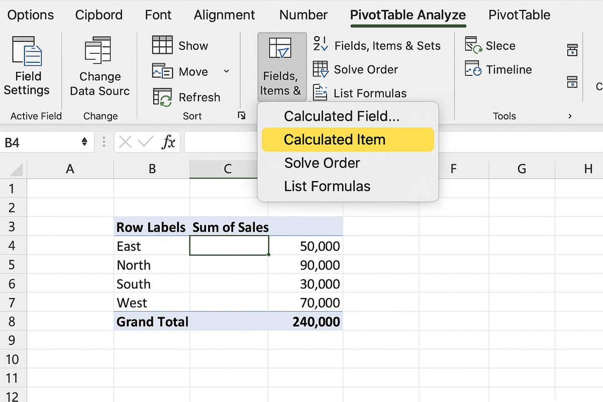
3. Click Fields, Items & Sets in the Calculations group, then select Calculated Field… from the dropdown menu.



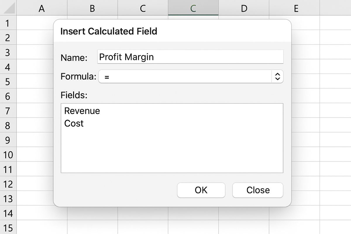
4. In the Insert Calculated Field dialog box, type Profit Margin in the Name field.



5. In the Formula box, enter the formula = (Revenue - Cost) / Revenue. Use the exact field names as they appear in your Pivot Table fields list.
6. Click Add and then OK to insert the calculated field into your Pivot Table.
7. Observe the new Profit Margin field added to the Values area of your Pivot Table.
8. To format the Profit Margin as a percentage, right-click any value in the Profit Margin column, select Value Field Settings, then click Number Format.
9. Choose Percentage and set the desired decimal places (e.g., 2), then click OK twice to apply the formatting.
10. If you update your source data, click Refresh on the PivotTable Analyze tab to update the calculated field results accordingly.

Tips for Using Calculated Fields Effectively

Remember that calculated fields operate on the aggregated data in your Pivot Table, not on the individual source data rows. Use them to create ratios, differences, or any other metric that helps you gain insights from your summarized data.

Conclusion

Mastering calculated fields in Pivot Tables empowers you to perform advanced data analysis directly within Excel, saving time and improving your reporting capabilities.