Mastering the Excel PIVOTBY Function for Advanced Data Summarization and Automation

The PIVOTBY function in Excel is a powerful tool designed to simplify complex data summarization tasks. By leveraging this function, users can automate the creation of PivotTables and gain deeper insights into their datasets with minimal manual effort.

In this article, we will explore the syntax, use cases, and advanced techniques to get the most out of PIVOTBY.

Understanding the PIVOTBY Function Syntax

The basic syntax of the PIVOTBY function is as follows:

=PIVOTBY(data, rows, columns, values, aggregation)

Where:

• data: The range of your source data.
• rows: The field(s) to use as row labels.
• columns: The field(s) to use as column labels.
• values: The field(s) to aggregate.
• aggregation: The aggregation function (e.g., SUM, COUNT).

Practical Steps to Create a Pivot Table Using PIVOTBY

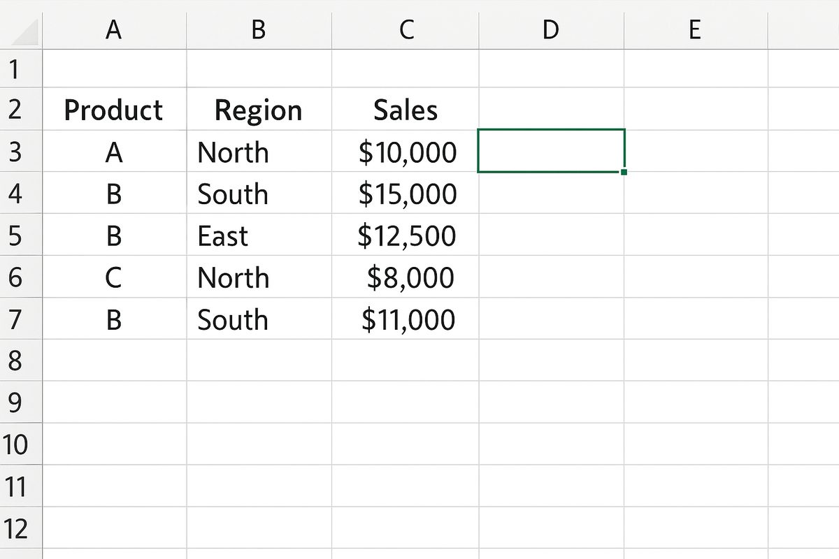
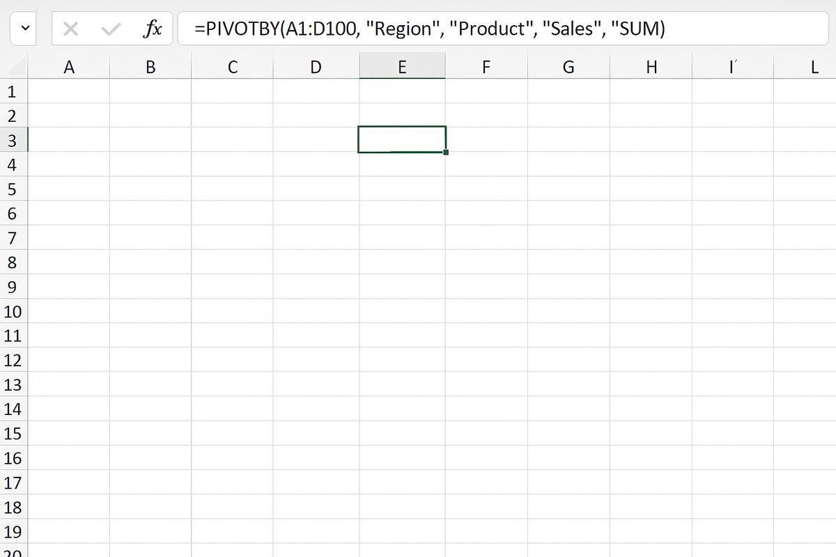
1. Select the range A1:D100 in your worksheet, which contains your source data including columns “Region”, “Product”, “Sales”, and “Date”.
2. Click on an empty cell where you want the pivot table output to appear, for example, cell F2.
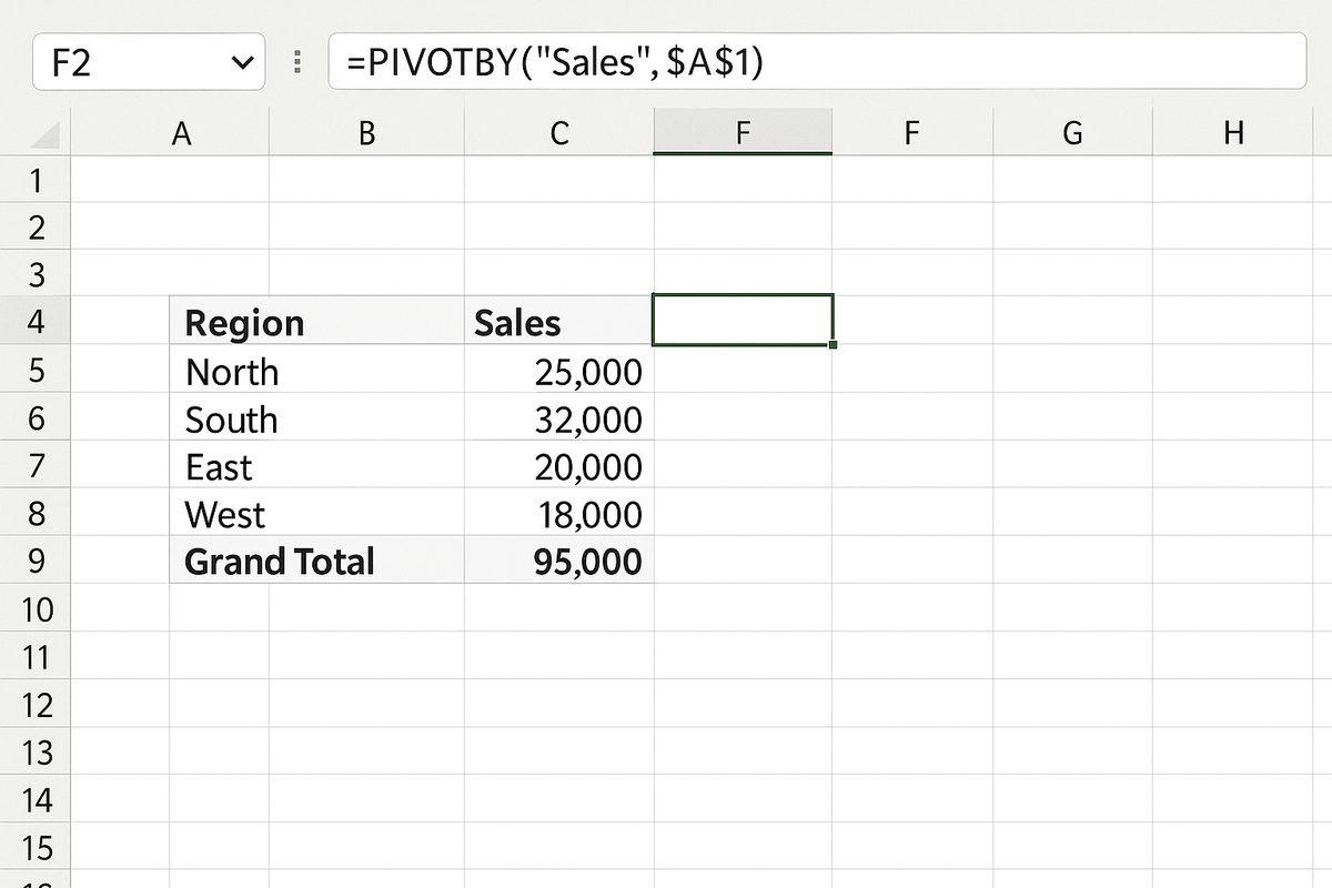
3. Enter the formula: =PIVOTBY(A1:D100, "Region", "Product", "Sales", "SUM") and press Enter.
4. Excel will generate a summarized table showing the sum of sales for each product by region.
5. To refresh the pivot table after updating the source data, select the cell with the PIVOTBY formula and press F9 to recalculate.



6. Optionally, format the resulting pivot table: select the range starting at F2, then go to the Home tab and apply Currency format to the sales values.
7. Inspect the pivot table to verify that the sales totals correspond correctly to each region and product combination.

Advanced Use Cases

Beyond basic summarization, PIVOTBY can be combined with other functions like FILTER and SORT to create dynamic reports that update automatically based on criteria you specify.

For example, you can filter sales data for a specific date range before summarizing, or sort the pivot results by total sales descending.

Conclusion

Mastering the PIVOTBY function empowers Excel users to automate data summarization tasks efficiently. By following the steps outlined and experimenting with different parameters, you can create customized pivot reports tailored to your analytical needs.