How to Use Slicers in Pivot Tables for Interactive Filtering

Introduction

Pivot tables are one of Excel’s most powerful features, allowing users to summarize, analyze, and present large datasets easily. However, when dealing with complex data, filtering becomes essential to focus on specific segments. This is where pivot table slicers come in handy. Slicers provide a user-friendly, visual method for filtering pivot table data interactively. In this article, we will explore how to use slicers effectively in pivot tables, enhance your data analysis experience, and walk you through practical examples.

What Are Pivot Table Slicers?

Slicers are visual filter controls introduced in Excel 2010 to make pivot table filtering more intuitive. Unlike traditional filter drop-downs, slicers display filter options as clickable buttons, making it easier to see which filters are applied at a glance. They are especially useful when sharing reports with others who may not be familiar with pivot table filters.

Benefits of Using Pivot Table Slicers

• Visual and intuitive filtering: Easily identify which data is selected.
• Quick filtering: Filter data with a single click without navigating drop-down menus.
• Multiple slicers control: Use several slicers for different fields simultaneously.
• Cleaner dashboards: Create interactive reports and dashboards with a professional look.

How to Insert a Slicer in a Pivot Table

Follow these steps to add a slicer to your pivot table:

1. Click anywhere inside your pivot table to activate the PivotTable Tools on the ribbon.
2. Go to the Analyze tab (or PivotTable Analyze in newer Excel versions).



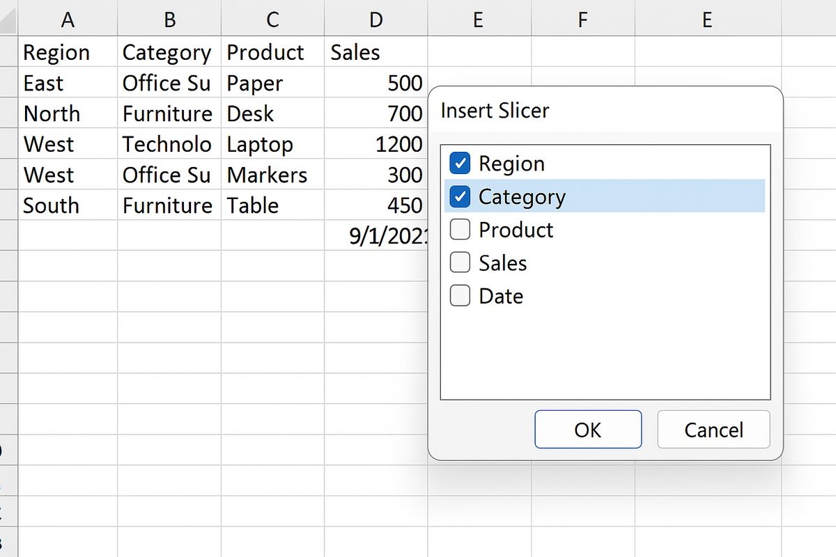
3. Click on Insert Slicer in the Filter group.
4. A dialog box will appear displaying all available fields from your pivot table’s data source.
5. Select the fields you want slicers for and click OK.
6. The slicer(s) will appear on your worksheet as clickable boxes representing the unique items in the selected field(s).

Practical Example: Using Slicers to Filter Sales Data

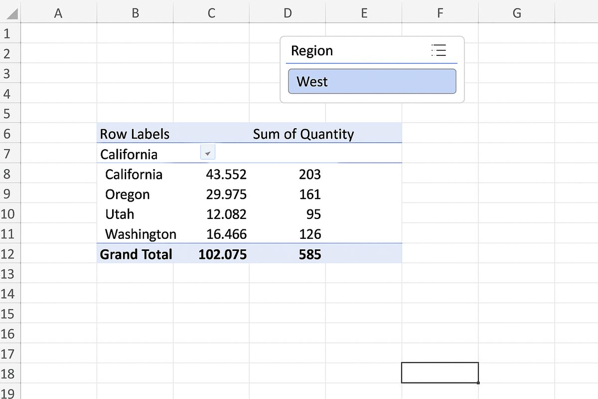
Imagine you have a pivot table summarizing sales data by region, product category, and date. You want to quickly filter by region and category without navigating multiple filter menus.

Step 1: Insert slicers for the Region and Category fields.

Step 2: Click on a slicer button corresponding to the desired region, for example, “West”. The pivot table will instantly update to show sales data for the West region only.

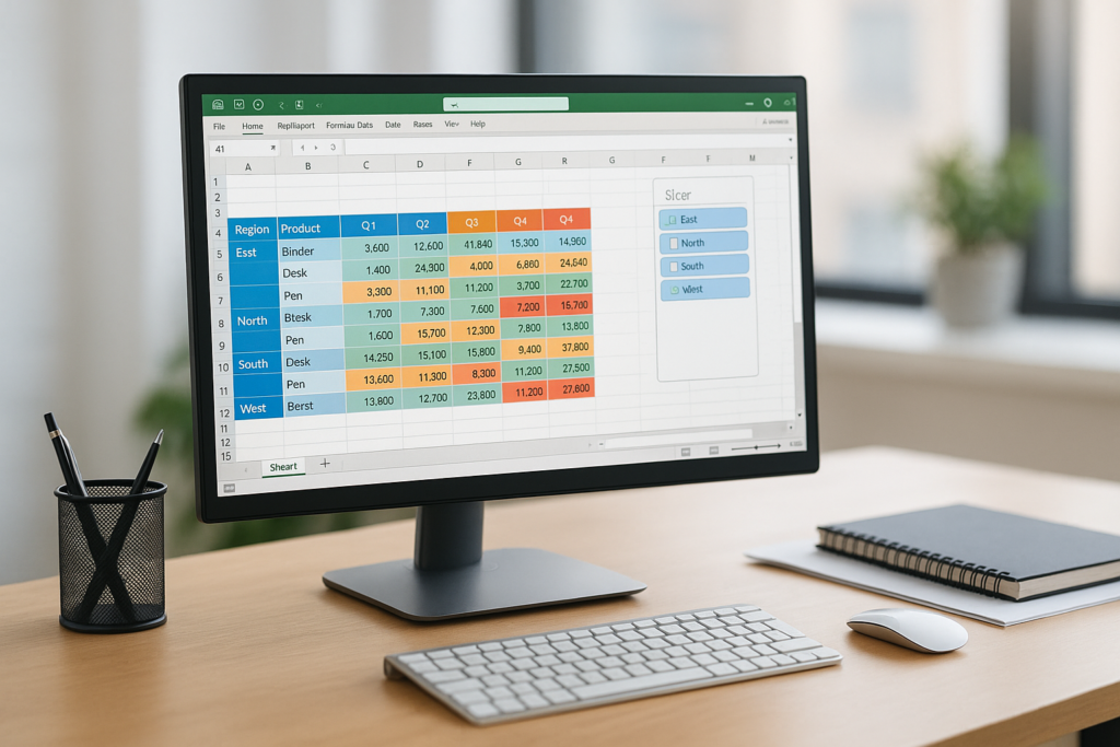
Step 3: Click on a category in the Category slicer, for example, “Electronics”; now the pivot table shows sales filtered by West region and Electronics category simultaneously.

Step 4: To clear a filter, click the filter icon (funnel with a red cross) at the top right of each slicer.

Customizing Slicers for Better Usability

You can customize slicers to improve usability and appearance:

• Resize: Drag the edges to resize the slicer buttons.
• Change columns: Display buttons in multiple columns for a more compact slicer.
• Change style: Use the Slicer Styles gallery on the ribbon to change colors and formatting.
• Align and arrange: Use Excel’s alignment tools to neatly arrange multiple slicers.

Using Slicers with Multiple Pivot Tables

You can connect one slicer to control multiple pivot tables if they share the same data source. This is ideal for dashboards that show different views of the same data.

How to connect a slicer to multiple pivot tables:

1. Insert a slicer for one pivot table as usual.
2. Click the slicer to activate the Slicer Tools ribbon.
3. Click Report Connections (or Pivot Table Connections).
4. In the dialog box, check all pivot tables you want the slicer to control.
5. Click OK.

Now, filtering with the slicer will update all connected pivot tables simultaneously.

Advanced Tips for Pivot Table Slicers

• Use Timelines: For date fields, consider using a Timeline slicer, which provides a dynamic and interactive way to filter dates.
• Keyboard shortcuts: Use keyboard navigation to select slicer buttons quickly.
• VBA automation: Automate slicer control through macros to streamline repetitive tasks.
• Keep slicers visible: Pin slicers in dashboards or freeze panes to keep filters accessible while scrolling.

Common Issues and Troubleshooting

• Slicer not filtering pivot table: Ensure the slicer is connected to the correct pivot table or tables.
• Slicer buttons missing: Refresh your pivot table if data has changed.
• Slow performance: Too many slicers or very large data sets might slow down Excel; consider limiting slicers or optimizing data.

Conclusion

Pivot table slicers are an essential tool for making your Excel data analysis more interactive and accessible. They simplify filtering by providing clear, clickable options that everyone can use, from beginners to advanced users. By integrating slicers into your pivot tables and dashboards, you improve both the usability and the visual appeal of your reports. Practice adding and customizing slicers in your pivot tables to unlock the full potential of Excel’s interactive filtering capabilities.

Related Articles

• Pivot Tables Tutorial: A Beginner’s Guide to Summarizing Data
• What Is a Pivot Table and How Can It Help You Analyze Data?
• How to Create a Pivot Table in Excel Step-by-Step
• Understanding Pivot Table Fields: Rows, Columns, Filters, and Values Explained
• Advanced Pivot Table Techniques to Master Data Analysis