Applying Conditional Formatting to Pivot Tables in Excel

Introduction

Pivot tables are powerful tools in Excel that allow users to summarize, analyze, explore, and present large amounts of data quickly. While pivot tables provide excellent ways to organize data, applying conditional formatting enhances their visual appeal and makes data insights clearer. This article guides you through the process of applying conditional formatting to pivot tables in Excel, offering practical examples to maximize your data analysis capabilities.

What is Pivot Table Conditional Formatting?

Conditional formatting in Excel is a feature that changes the appearance of cells based on specific criteria. When applied to pivot tables, conditional formatting highlights data dynamically according to rules you set, making it easier to spot trends, outliers, or significant values within your summarized data.

Benefits of Using Conditional Formatting on Pivot Tables

• Improved data visualization: Highlight important data points such as high or low values, duplicates, or specific ranges.
• Quick insight: Easily identify trends, patterns, or anomalies without scanning through large datasets manually.
• Customization: Tailor pivot tables to different audiences by emphasizing relevant information.
• Dynamic updates: Formatting adjusts automatically as your pivot table data changes.

How to Apply Conditional Formatting to Pivot Tables

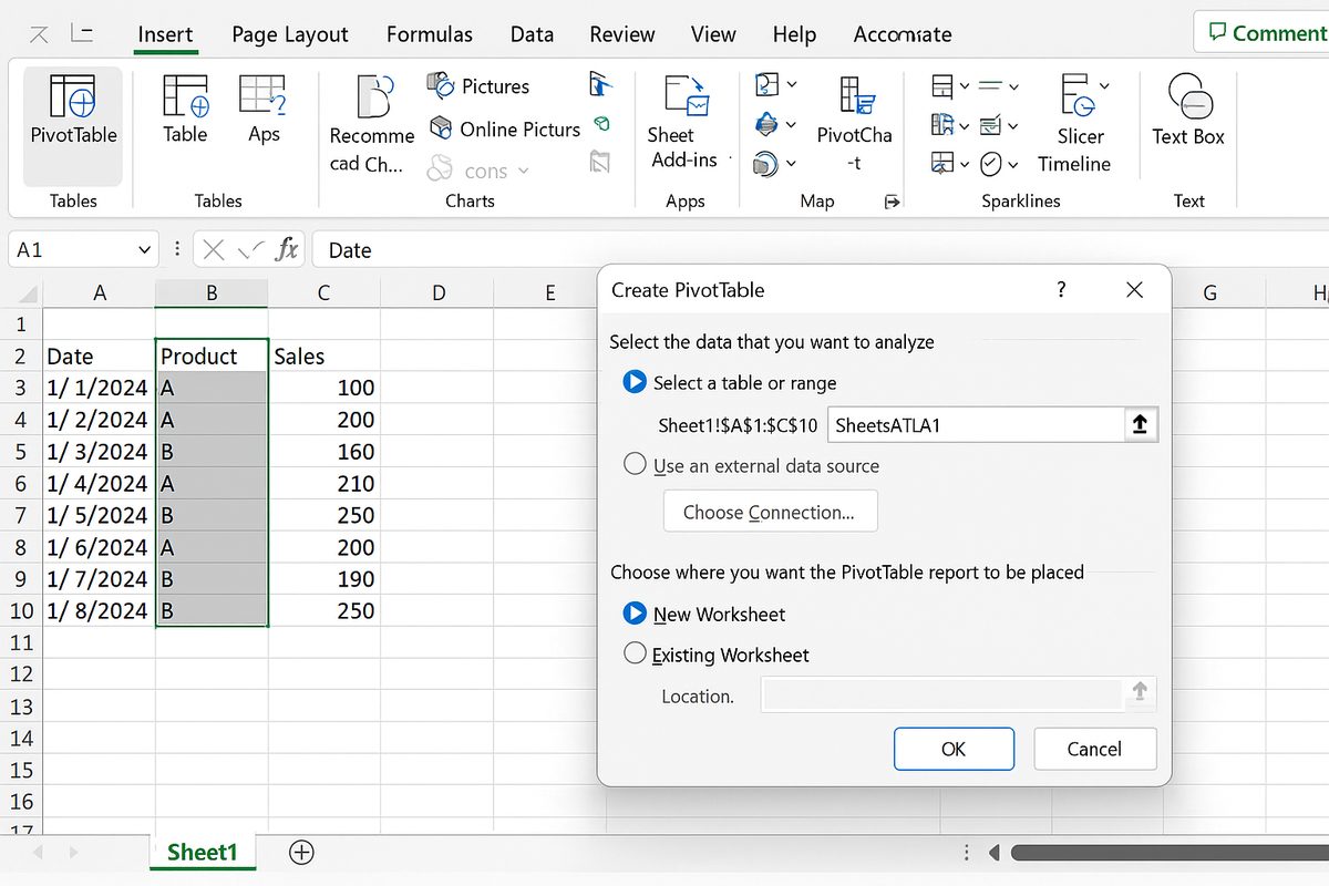
Step 1: Create Your Pivot Table

First, prepare a dataset and insert a pivot table:

1. Select your data range.
2. Go to Insert > PivotTable.



3. Choose where to place the pivot table (new worksheet or existing worksheet).
4. Drag and drop fields into Rows, Columns, and Values areas to summarize your data.

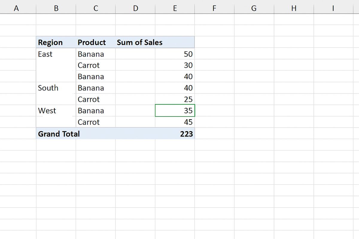
Step 2: Select the Cells in the Pivot Table

Click any cell inside the pivot table that you want to format. Usually, you will apply conditional formatting to the data area (values) rather than the row or column labels.

Step 3: Open Conditional Formatting

Navigate to the Home tab on the ribbon, and click Conditional Formatting. You will see several options such as Highlight Cells Rules, Top/Bottom Rules, and Data Bars.

Step 4: Choose a Rule Type

Pick the appropriate formatting rule based on your needs. For example:

• Highlight Cells Rules: Format cells greater than a certain value.
• Color Scales: Apply gradient colors based on cell values.
• Data Bars: Add bars inside cells representing values.

Step 5: Set the Formatting Criteria

Define the conditions for your formatting rule. For instance, you might want to highlight sales figures above $10,000 in green.

Step 6: Apply the Rule

Click OK to apply the conditional formatting. Your pivot table will now visually highlight the cells meeting your criteria.

Practical Examples

Example 1: Highlight Top 10 Sales Values

1. Create a pivot table summarizing sales data by product.
2. Select the sales values area.
3. Go to Home > Conditional Formatting > Top/Bottom Rules > Top 10 Items.
4. Set formatting (e.g., bold font with light green fill).
5. Click OK to highlight the top 10 sales values.

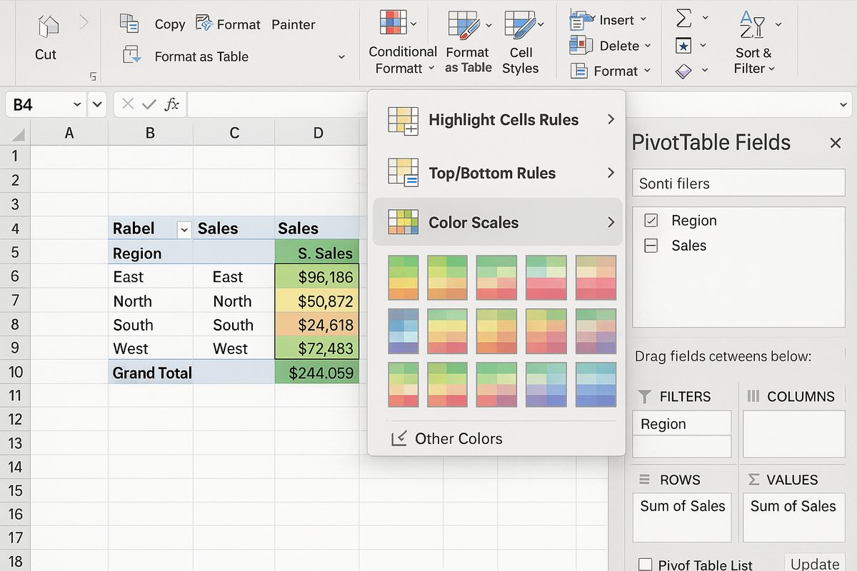
Example 2: Apply Color Scales to Show Sales Range

1. Select the values area in your pivot table.
2. Go to Conditional Formatting > Color Scales.



3. Choose a gradient scale such as green-yellow-red.
4. The highest sales will appear green and the lowest red, with shades in between.

Example 3: Highlight Duplicate Values in a Pivot Table

1. Select the relevant pivot table area.
2. Choose Conditional Formatting > Highlight Cells Rules > Duplicate Values.
3. Set a formatting style, such as red fill with dark red text.
4. Duplicates will be highlighted immediately, helping you identify repeated entries.

Tips and Best Practices

• Use pivot table specific rules: Excel allows you to apply conditional formatting rules that adjust dynamically as the pivot table updates. Use the “All cells showing ” option to ensure formatting applies only to visible pivot data.
• Avoid over-formatting: Too many colors or styles can confuse users. Keep formatting simple and meaningful.
• Test formatting with sample changes: Modify your pivot table filters or data to check if conditional formatting updates correctly.
• Use custom formulas: For advanced scenarios, create formula-based conditional formatting rules to handle complex conditions.

Common Challenges and Solutions

Formatting Not Applying Correctly After Refresh

Sometimes, conditional formatting may seem lost after refreshing the pivot table. To prevent this, ensure you apply formatting using the “All cells showing” option in the conditional formatting rule manager. This links the formatting to the pivot table’s visible cells, preserving it after refresh.

Formatting Only Part of the Pivot Table

Make sure to select the entire data range or the specific fields you want to format rather than just a single cell. Applying conditional formatting to the whole pivot table data area ensures consistent results.

Conclusion

Applying conditional formatting to pivot tables in Excel is an effective way to enhance data visualization and make your reports more insightful and user-friendly. By leveraging Excel’s built-in conditional formatting tools, you can highlight key data points dynamically and customize your pivot tables to fit your analytical needs. Using the practical examples and tips provided, you can confidently apply pivot table conditional formatting to improve your data analysis process.

Related Articles

• Pivot Tables Tutorial: A Beginner’s Guide to Summarizing Data
• What Is a Pivot Table and How Can It Help You Analyze Data?
• How to Create a Pivot Table in Excel Step-by-Step
• Understanding Pivot Table Fields: Rows, Columns, Filters, and Values Explained
• Advanced Pivot Table Techniques to Master Data Analysis