Error Handling in XLOOKUP: Tips to Avoid Common Mistakes

Introduction
XLOOKUP is one of the most powerful functions in Excel, designed to replace older lookup functions like VLOOKUP and HLOOKUP by offering more flexibility and accuracy. However, like any advanced function, users often encounter errors that can disrupt workflows and lead to incorrect data retrieval. This comprehensive guide focuses on XLOOKUP error handling, providing tips and practical examples to help you avoid common mistakes and master advanced lookup techniques.
Understanding Common XLOOKUP Errors
Before diving into error handling, it’s important to understand the typical errors that XLOOKUP users face. Some of the most frequent errors include:
#N/A: The lookup value is not found in the lookup array.#VALUE!: Occurs when the arguments provided to XLOOKUP are invalid or of incorrect type.#REF!: Happens when referencing invalid ranges or deleted sheets.
Awareness of these errors helps in crafting robust formulas that anticipate and manage them effectively.
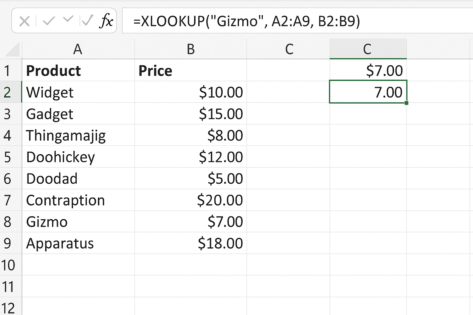
Basic XLOOKUP Syntax Refresher
For clarity, here is the basic syntax of XLOOKUP:
=XLOOKUP(lookup_value, lookup_array, return_array, [if_not_found], [match_mode], [search_mode])The optional if_not_found argument is key to handling errors gracefully.
Using the IF_NOT_FOUND Argument to Handle Errors
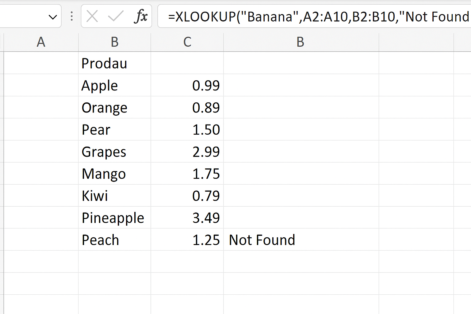
The if_not_found parameter allows you to specify a custom message or value when the lookup value doesn’t exist, instead of returning the default #N/A error.
Example:
=XLOOKUP("Banana", A2:A10, B2:B10, "Not Found")This formula looks for “Banana” in the range A2:A10 and returns the corresponding value from B2:B10. If “Banana” is missing, it will display “Not Found” instead of #N/A.
Combining XLOOKUP with IFERROR for Advanced Error Handling
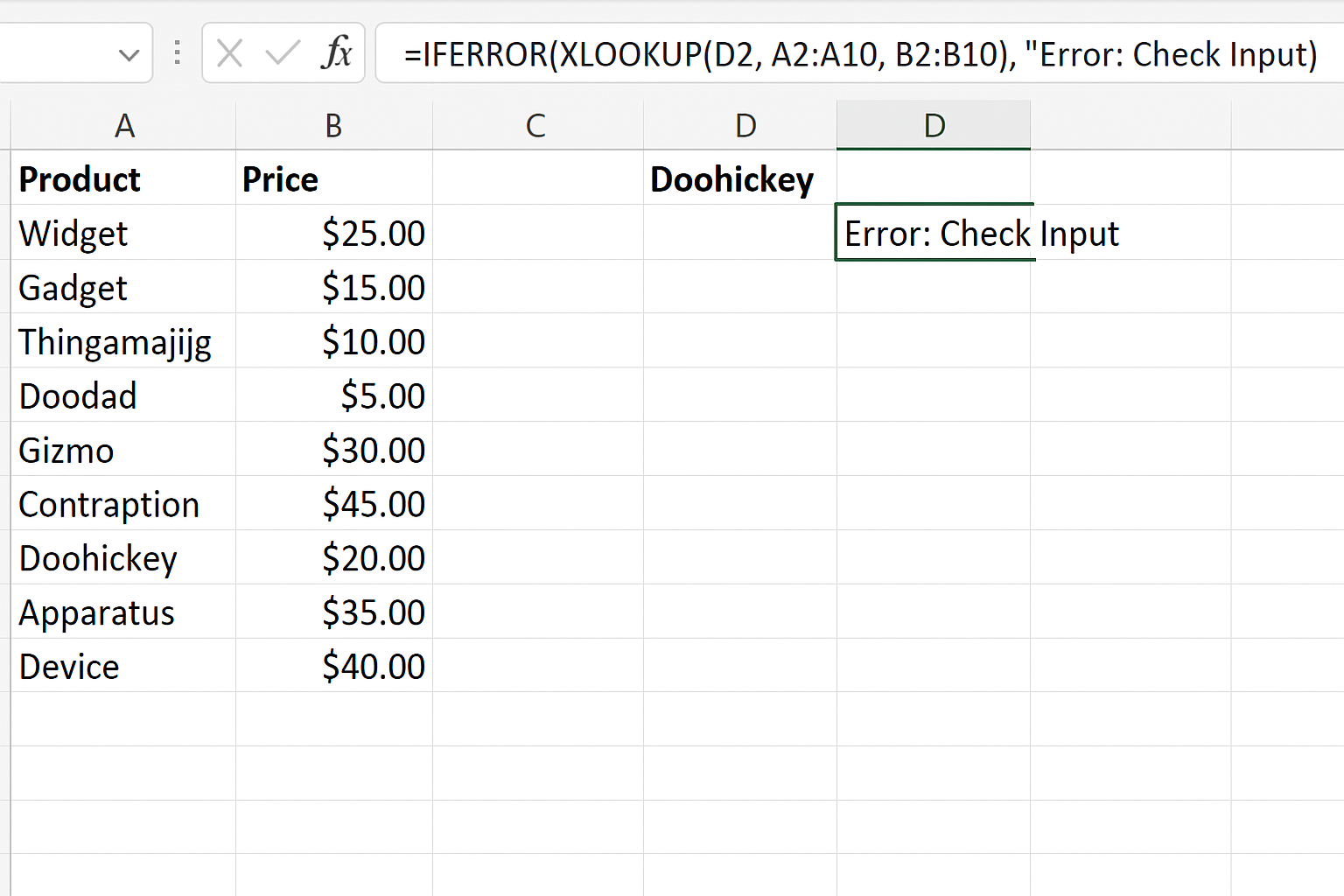
While if_not_found handles missing data, other errors might still occur. Wrapping XLOOKUP inside the IFERROR function can catch any error and return a custom result.
Example:
=IFERROR(XLOOKUP(D2, A2:A10, B2:B10), "Error: Check Input")This formula returns the lookup result if found; otherwise, it shows “Error: Check Input” for any error encountered.
Practical Tips to Avoid Common XLOOKUP Mistakes
1. Ensure Lookup and Return Arrays Are Equal Length
Mismatched array lengths cause #VALUE! errors. Always verify that lookup_array and return_array cover the same number of rows or columns.
2. Use Exact Match Mode for Precise Results
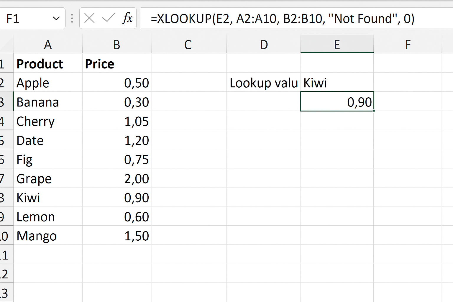
By default, XLOOKUP uses exact match mode (match_mode=0). Explicitly setting this can prevent unexpected errors.
=XLOOKUP(E2, A2:A10, B2:B10, "Not Found", 0)3. Handle Case Sensitivity
XLOOKUP is not case-sensitive by default. To perform case-sensitive lookups, combine XLOOKUP with helper functions like EXACT.
4. Avoid Circular References
Be careful when XLOOKUP formulas reference cells that depend on the formula’s output, as this can cause calculation errors.
Example: Building a Robust Product Price Lookup
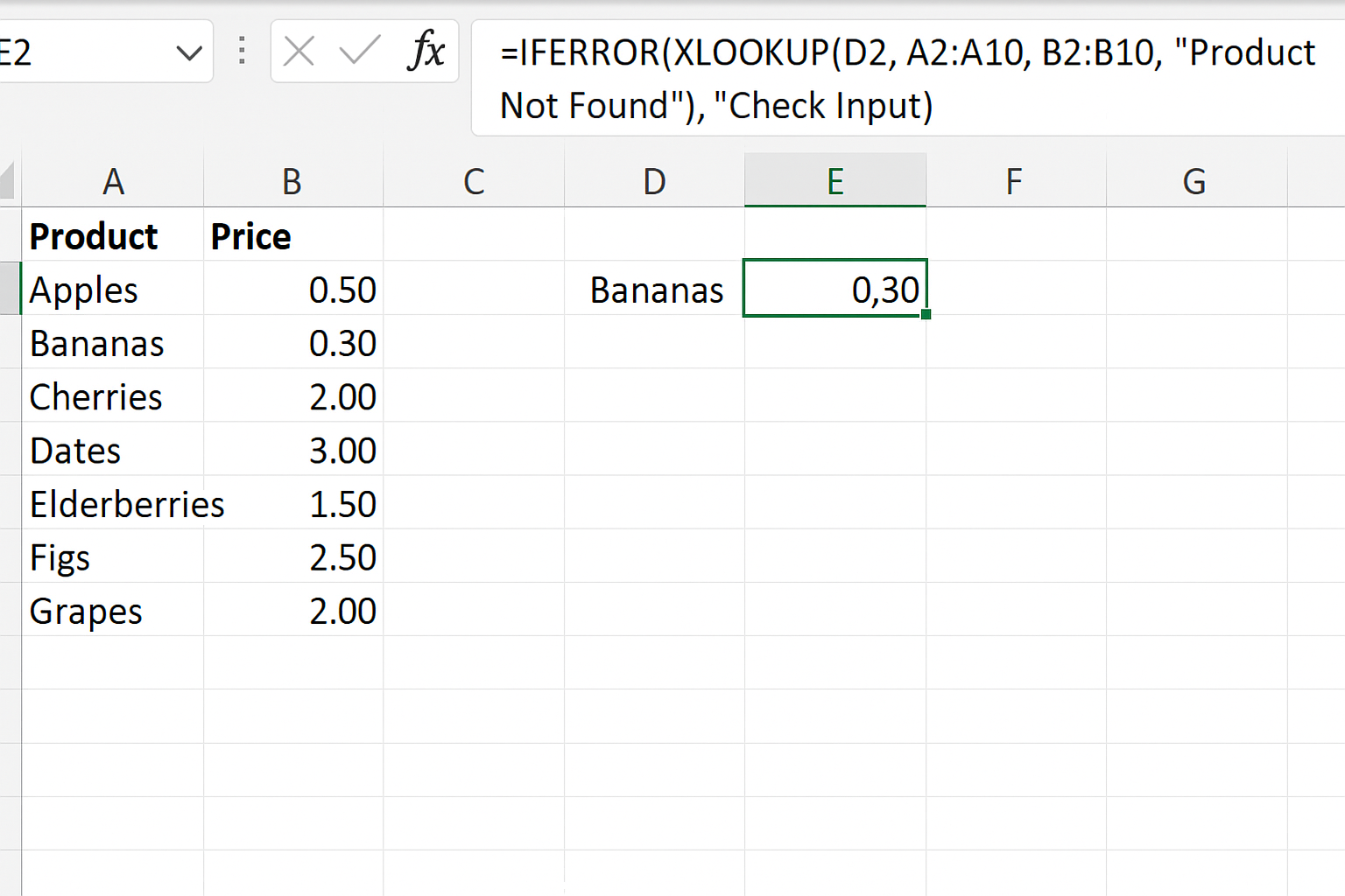
Consider a product list in columns A (Product Name) and B (Price). You want to retrieve prices based on user input in cell D2.
=IFERROR(XLOOKUP(D2, A2:A10, B2:B10, "Product Not Found"), "Check Input")This formula first attempts to find the product price. If the product is missing, it returns “Product Not Found.” If there’s any other error, it advises to check the input.
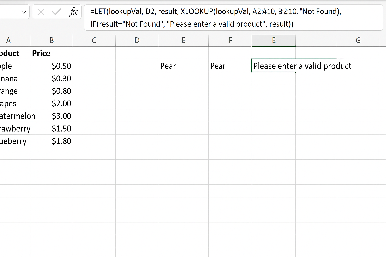
Advanced Error Handling: Using LET with XLOOKUP
For complex workbooks, the LET function improves readability and performance by storing intermediate calculations.
=LET(lookupVal, D2,
  result, XLOOKUP(lookupVal, A2:A10, B2:B10, "Not Found"),
  IF(result="Not Found", "Please enter a valid product", result))
This formula stores the lookup value and result, then checks if the product was found, providing a user-friendly message if not.
FAQ
Below are some frequently asked questions about XLOOKUP error handling.
Related Articles
- Getting Started with XLOOKUP in Excel: A Beginner’s Guide
- How to Use XLOOKUP in Excel to Find Data Quickly
- Understanding XLOOKUP Syntax and Parameters in Excel
- How to Use XLOOKUP with Multiple Criteria in Excel
- XLOOKUP vs VLOOKUP: Which Excel Function Should You Use?
Want practical Excel help?
Support free Excel tutorials, get weekly tips, or contact us for Excel programming, VBA, Power Query, dashboards, and automation work.