Understanding XLOOKUP Syntax and Parameters in Excel

Introduction
Excel’s XLOOKUP function is a powerful and flexible tool designed to replace older lookup functions like VLOOKUP and HLOOKUP. Understanding the XLOOKUP syntax and its parameters is crucial for efficiently searching and retrieving data within a spreadsheet. This comprehensive guide will walk you through the syntax, parameters, practical examples, and tips to leverage XLOOKUP for your data analysis needs.
What is XLOOKUP?
XLOOKUP is a lookup function introduced in Excel 365 and Excel 2019 that allows you to search a range or array, find the matching value, and return the corresponding result from another range or array. It addresses many limitations of VLOOKUP, such as the inability to lookup values to the left and the need for sorted data.
XLOOKUP Syntax
The basic syntax of the XLOOKUP function is:
XLOOKUP(lookup_value, lookup_array, return_array, [if_not_found], [match_mode], [search_mode])
Let’s break down each parameter:
- lookup_value: The value you want to search for.
- lookup_array: The array or range where Excel searches for the lookup_value.
- return_array: The array or range that contains the values you want returned.
- [if_not_found]: Optional. The value to return if no match is found. If omitted, Excel returns an #N/A error.
- [match_mode]: Optional. Specifies the type of match to perform:
- 0 – Exact match (default)
- -1 – Exact match or next smaller item
- 1 – Exact match or next larger item
- 2 – Wildcard match (supports *, ?, ~)
- [search_mode]: Optional. Specifies the search direction:
- 1 – Search first-to-last (default)
- -1 – Search last-to-first
- 2 – Binary search ascending (lookup_array must be sorted ascending)
- -2 – Binary search descending (lookup_array must be sorted descending)
Detailed Explanation of Parameters
lookup_value
This is the value that you want to find in the lookup_array. It can be a number, text, logical value, or even a cell reference containing the value.
lookup_array
Defines where Excel will search for the lookup_value. It needs to be a one-dimensional range or array. Unlike VLOOKUP, this does not need to be the leftmost column.
return_array
Once the lookup_value is found, Excel returns the corresponding value from this array or range, which must be the same size as lookup_array.
[if_not_found]
If the lookup_value is not found in the lookup_array, this optional parameter allows you to specify what to return instead of the default #N/A error.
[match_mode]
This parameter controls how Excel matches the lookup_value with values in the lookup_array. You can perform exact matches, approximate matches, or wildcard searches to fit varied needs.
[search_mode]
Defines the order of the search. You can search from the beginning to end, from the end to beginning, or use binary search for sorted data for faster performance.
Practical Examples
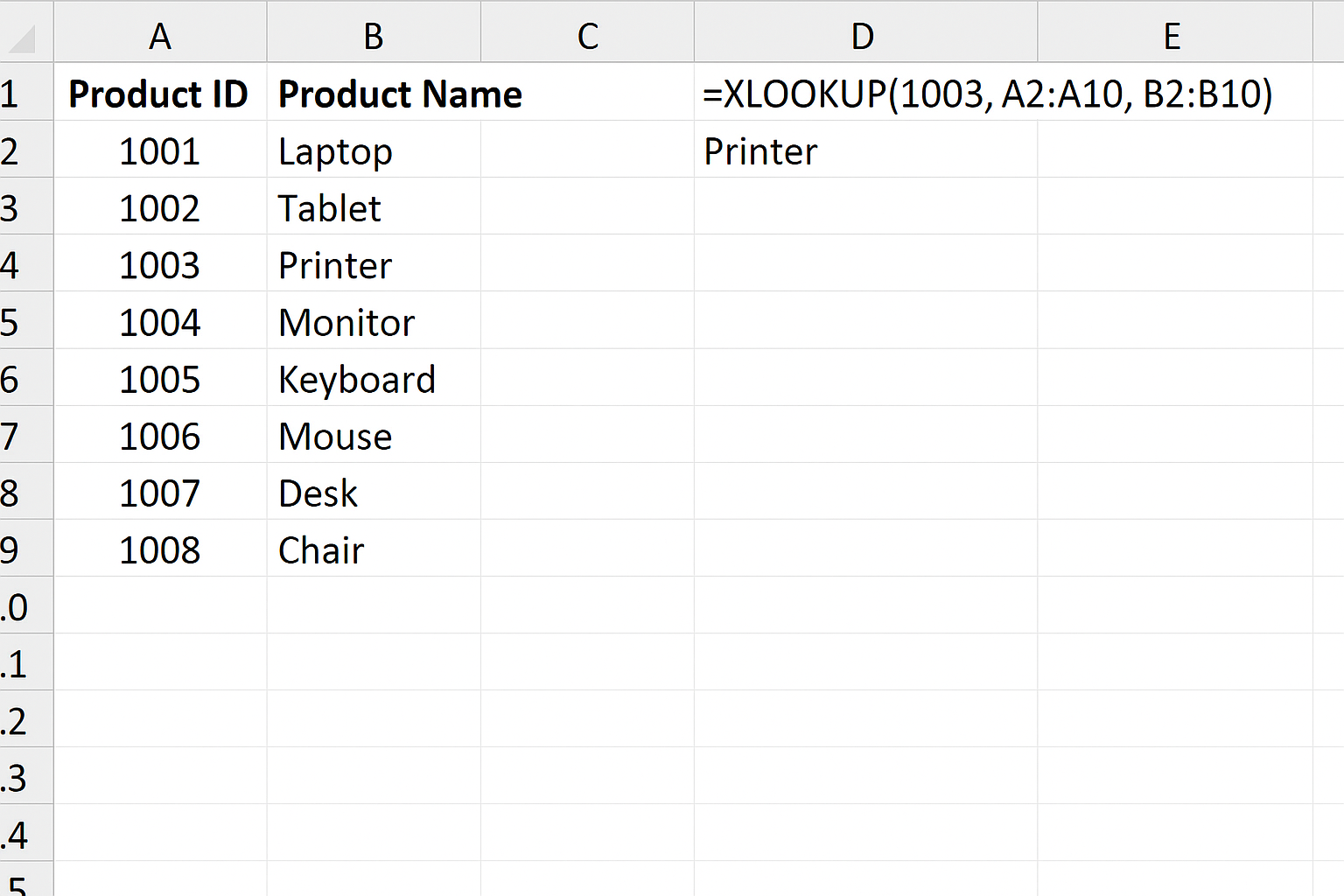
Example 1: Basic Exact Match
Assume you have a list of product IDs in column A and product names in column B. To find the product name for a given product ID, use:
=XLOOKUP(1003, A2:A10, B2:B10)
This formula looks for the value 1003 in A2:A10 and returns the corresponding product name from B2:B10.
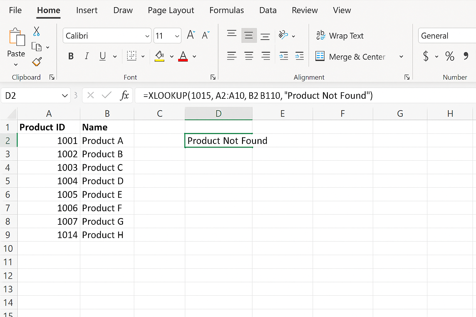
Example 2: Handling Not Found Values
If the product ID might not be in the list, include the if_not_found parameter to show a friendly message instead of an error:
=XLOOKUP(1015, A2:A10, B2:B10, "Product Not Found")
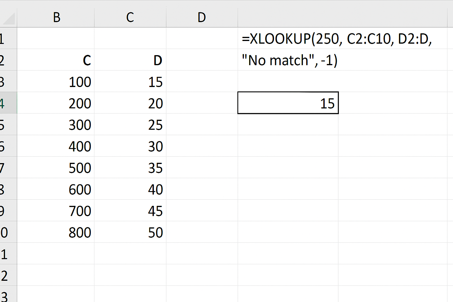
Example 3: Approximate Match
To find the closest smaller match (e.g., for pricing tiers), use match_mode = -1:
=XLOOKUP(250, C2:C10, D2:D10, "No match", -1)
This looks for 250 in C2:C10 and returns the corresponding value from D2:D10, or the next smaller value if an exact match is not found.
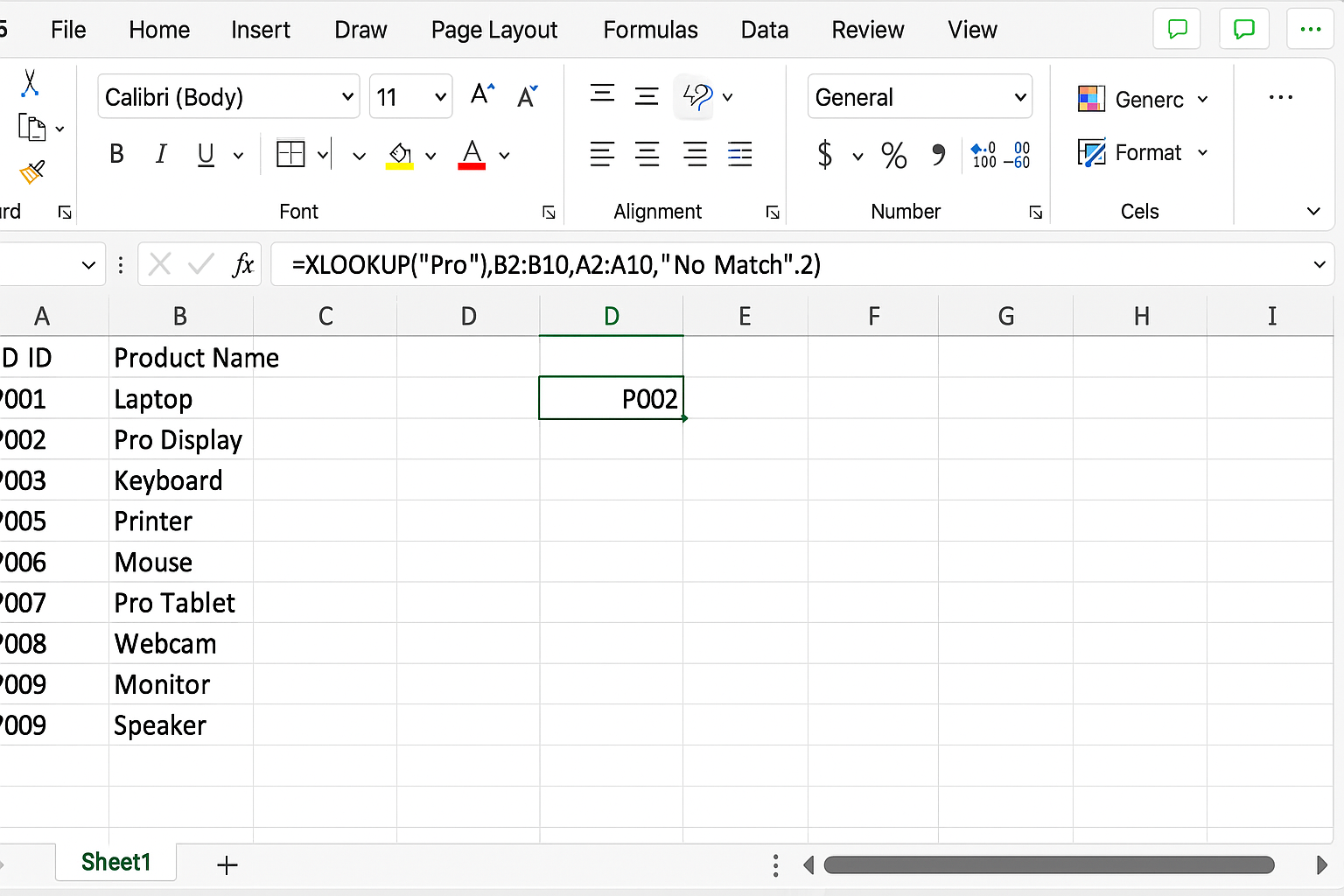
Example 4: Wildcard Match
You can search text using wildcards. For example, to find any product name starting with “Pro”:
=XLOOKUP("Pro*", B2:B10, A2:A10, "No Match", 2)
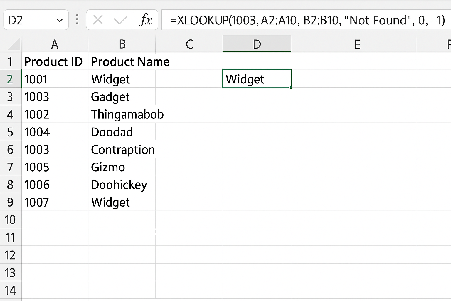
Example 5: Reverse Search
To find the last occurrence of a value, use search_mode = -1:
=XLOOKUP(1003, A2:A10, B2:B10, "Not Found", 0, -1)
Tips for Using XLOOKUP Syntax Effectively
- Always ensure that the lookup_array and return_array have the same dimensions.
- Use the if_not_found parameter to avoid errors and improve user experience.
- Leverage match_mode for flexible matching criteria.
- Use search_mode to optimize performance when working with large, sorted datasets.
Common Errors and Troubleshooting
- #N/A: Lookup value not found and if_not_found parameter is omitted.
- #VALUE!: Mismatch in array sizes between lookup_array and return_array.
- #REF!: Invalid references in parameters.
Conclusion
The XLOOKUP syntax is intuitive and versatile, making it the go-to function for lookup operations in Excel. By understanding each parameter and applying practical examples, you can efficiently retrieve data, handle errors gracefully, and perform complex searches with ease. Mastering XLOOKUP empowers you to create more dynamic and robust spreadsheets.
Related Articles
- Getting Started with XLOOKUP in Excel: A Beginner’s Guide
- How to Use XLOOKUP in Excel to Find Data Quickly
- How to Use XLOOKUP with Multiple Criteria in Excel
- Error Handling in XLOOKUP: Tips to Avoid Common Mistakes
- XLOOKUP vs VLOOKUP: Which Excel Function Should You Use?
Want practical Excel help?
Support free Excel tutorials, get weekly tips, or contact us for Excel programming, VBA, Power Query, dashboards, and automation work.